Summit User Guide
Warning
This system was decommissioned on November 15, 2024 and is no longer online. Information here is presented as an archive and is no longer updated.
Summit Documentation Resources
In addition to this Summit User Guide, there are other sources of documentation, instruction, and tutorials that could be useful for Summit users.
The OLCF Training Archive provides a list of previous training events, including multi-day Summit Workshops. Some examples of topics addressed during these workshops include using Summit’s NVME burst buffers, CUDA-aware MPI, advanced networking and MPI, and multiple ways of programming multiple GPUs per node. You can also find simple tutorials and code examples for some common programming and running tasks in our Github tutorial page .
System Overview
Summit is an IBM system located at the Oak Ridge Leadership Computing Facility. With a theoretical peak double-precision performance of approximately 200 PF, it is one of the most capable systems in the world for a wide range of traditional computational science applications. It is also one of the “smartest” computers in the world for deep learning applications with a mixed-precision capability in excess of 3 EF.
Summit Nodes
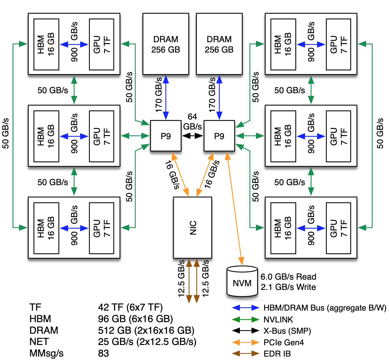
The basic building block of Summit is the IBM Power System AC922 node. Each of the approximately 4,600 compute nodes on Summit contains two IBM POWER9 processors and six NVIDIA Tesla V100 accelerators and provides a theoretical double-precision capability of approximately 40 TF. Each POWER9 processor is connected via dual NVLINK bricks, each capable of a 25GB/s transfer rate in each direction.
Most Summit nodes contain 512 GB of DDR4 memory for use by the POWER9 processors, 96 GB of High Bandwidth Memory (HBM2) for use by the accelerators, and 1.6TB of non-volatile memory that can be used as a burst buffer. A small number of nodes (54) are configured as “high memory” nodes. These nodes contain 2TB of DDR4 memory, 192GB of HBM2, and 6.4TB of non-volatile memory.
The POWER9 processor is built around IBM’s SIMD Multi-Core (SMC). The processor provides 22 SMCs with separate 32kB L1 data and instruction caches. Pairs of SMCs share a 512kB L2 cache and a 10MB L3 cache. SMCs support Simultaneous Multi-Threading (SMT) up to a level of 4, meaning each physical core supports up to 4 Hardware Threads.
The POWER9 processors and V100 accelerators are cooled with cold plate technology. The remaining components are cooled through more traditional methods, although exhaust is passed through a back-of-cabinet heat exchanger prior to being released back into the room. Both the cold plate and heat exchanger operate using medium temperature water which is more cost-effective for the center to maintain than chilled water used by older systems.
Node Types
On Summit, there are three major types of nodes you will encounter: Login, Launch, and Compute. While all of these are similar in terms of hardware (see: Summit Nodes), they differ considerably in their intended use.
Node Type |
Description |
|---|---|
Login |
When you connect to Summit, you’re placed on a login node. This is the place to write/edit/compile your code, manage data, submit jobs, etc. You should never launch parallel jobs from a login node nor should you run threaded jobs on a login node. Login nodes are shared resources that are in use by many users simultaneously. |
Launch |
When your batch script (or interactive batch job) starts running, it will execute on a Launch Node. (If you were a user of Titan, these are similar in function to service nodes on that system). All commands within your job script (or the commands you run in an interactive job) will run on a launch node. Like login nodes, these are shared resources so you should not run multiprocessor/threaded programs on Launch nodes. It is appropriate to launch the jsrun command from launch nodes. |
Compute |
Most of the nodes on Summit are compute nodes. These are where your parallel job executes. They’re accessed via the jsrun command. |
Although the nodes are logically organized into different types, they
all contain similar hardware. As a result of this homogeneous
architecture there is not a need to cross-compile when building on a
login node. Since login nodes have similar hardware resources as compute
nodes, any tests that are run by your build process (especially by
utilities such as autoconf and cmake) will have access to the
same type of hardware that is on compute nodes and should not require
intervention that might be required on non-homogeneous systems.
Note
Login nodes have (2) 16-core Power9 CPUs and (4) V100 GPUs. Compute nodes have (2) 22-core Power9 CPUs and (6) V100 GPUs.
System Interconnect
Summit nodes are connected to a dual-rail EDR InfiniBand network providing a node injection bandwidth of 23 GB/s. Nodes are interconnected in a Non-blocking Fat Tree topology. This interconnect is a three-level tree implemented by a switch to connect nodes within each cabinet (first level) along with Director switches (second and third level) that connect cabinets together.
File Systems
Summit is connected to an IBM Spectrum Scale™ filesystem named Alpine2. Summit also has access to the center-wide NFS-based filesystem (which provides user and project home areas) and has access to the center’s Nearline archival storage system (Kronos) for user and project archival storage.
Operating System
Summit is running Red Hat Enterprise Linux (RHEL) version 8.2.
Hardware Threads
The IBM POWER9 processor supports Hardware Threads. Each of the POWER9’s physical cores has 4 “slices”. These slices provide Simultaneous Multi Threading (SMT) support within the core. Three SMT modes are supported: SMT4, SMT2, and SMT1. In SMT4 mode, each of the slices operates independently of the other three. This would permit four separate streams of execution (i.e. OpenMP threads or MPI tasks) on each physical core. In SMT2 mode, pairs of slices work together to run tasks. Finally, in SMT1 mode the four slices work together to execute the task/thread assigned to the physical core. Regardless of the SMT mode used, the four slices share the physical core’s L1 instruction & data caches. https://vimeo.com/283756938
GPUs
Each Summit Compute node has 6 NVIDIA V100 GPUs. The NVIDIA Tesla V100 accelerator has a peak performance of 7.8 TFLOP/s (double-precision) and contributes to a majority of the computational work performed on Summit. Each V100 contains 80 streaming multiprocessors (SMs), 16 GB (32 GB on high-memory nodes) of high-bandwidth memory (HBM2), and a 6 MB L2 cache that is available to the SMs. The GigaThread Engine is responsible for distributing work among the SMs and (8) 512-bit memory controllers control access to the 16 GB (32 GB on high-memory nodes) of HBM2 memory. The V100 uses NVIDIA’s NVLink interconnect to pass data between GPUs as well as from CPU-to-GPU. We provide a more in-depth look into the NVIDIA Tesla V100 later in the Summit Guide.
Connecting
To connect to Summit, ssh to summit.olcf.ornl.gov. For example:
ssh username@summit.olcf.ornl.gov
For more information on connecting to OLCF resources, see Connecting for the first time.
Data and Storage
For more information about center-wide file systems and data archiving available on Summit, please refer to the pages on Data Storage and Transfers.
Each compute node on Summit has a 1.6TB Non-Volatile Memory (NVMe) storage device (high-memory nodes have a 6.4TB NVMe storage device), colloquially known as a “Burst Buffer” with theoretical performance peak of 2.1 GB/s for writing and 5.5 GB/s for reading. The NVMes could be used to reduce the time that applications wait for I/O. More information can be found later in the Burst Buffer section.
Software
Visualization and analysis tasks should be done on the Andes cluster. There are a few tools provided for various visualization tasks, as described in the Visualization tools section of the Andes User Guide.
For a full list of software available at the OLCF, please see the Software section (coming soon).
Shell & Programming Environments
OLCF systems provide many software packages and scientific libraries pre-installed at the system-level for users to take advantage of. To facilitate this, environment management tools are employed to handle necessary changes to the shell. The sections below provide information about using these management tools on Summit.
Default Shell
A user’s default shell is selected when completing the User Account Request form. The chosen shell is set across all OLCF resources, and is the shell interface a user will be presented with upon login to any OLCF system. Currently, supported shells include:
bash
tcsh
csh
ksh
If you would like to have your default shell changed, please contact the OLCF User Assistance Center at help@nccs.gov.
Environment Management with Lmod
Environment modules are provided through Lmod, a Lua-based module system for
dynamically altering shell environments. By managing changes to the shell’s
environment variables (such as PATH, LD_LIBRARY_PATH, and
PKG_CONFIG_PATH), Lmod allows you to alter the software available in your
shell environment without the risk of creating package and version combinations
that cannot coexist in a single environment.
Lmod is a recursive environment module system, meaning it is aware of module compatibility and actively alters the environment to protect against conflicts. Messages to stderr are issued upon Lmod implicitly altering the environment. Environment modules are structured hierarchically by compiler family such that packages built with a given compiler will only be accessible if the compiler family is first present in the environment.
Note
Lmod can interpret both Lua modulefiles and legacy Tcl modulefiles. However, long and logic-heavy Tcl modulefiles may require porting to Lua.
General Usage
Typical use of Lmod is very similar to that of interacting with
modulefiles on other OLCF systems. The interface to Lmod is provided by
the module command:
Command |
Description |
|---|---|
module -t list |
Shows a terse list of the currently loaded modules. |
module avail |
Shows a table of the currently available modules |
module help <modulename> |
Shows help information about <modulename> |
module show <modulename> |
Shows the environment changes made by the <modulename> modulefile |
module spider <string> |
Searches all possible modules according to <string> |
module load <modulename> […] |
Loads the given <modulename>(s) into the current environment |
module use <path> |
Adds <path> to the modulefile search cache and |
module unuse <path> |
Removes <path> from the modulefile search cache and |
module purge |
Unloads all modules |
module reset |
Resets loaded modules to system defaults |
module update |
Reloads all currently loaded modules |
Note
Modules are changed recursively. Some commands, such as
module swap, are available to maintain compatibility with scripts
using Tcl Environment Modules, but are not necessary since Lmod
recursively processes loaded modules and automatically resolves
conflicts.
Searching for modules
Modules with dependencies are only available when the underlying dependencies,
such as compiler families, are loaded. Thus, module avail will only display
modules that are compatible with the current state of the environment. To search
the entire hierarchy across all possible dependencies, the spider
sub-command can be used as summarized in the following table.
Command |
Description |
|---|---|
module spider |
Shows the entire possible graph of modules |
module spider <modulename> |
Searches for modules named <modulename> in the graph of possible modules |
module spider <modulename>/<version> |
Searches for a specific version of <modulename> in the graph of possible modules |
module spider <string> |
Searches for modulefiles containing <string> |
Defining custom module collections
Lmod supports caching commonly used collections of environment modules on a
per-user basis in $HOME/.lmod.d. To create a collection called “NAME” from
the currently loaded modules, simply call module save NAME. Omitting “NAME”
will set the user’s default collection. Saved collections can be recalled and
examined with the commands summarized in the following table.
Command |
Description |
|---|---|
module restore NAME |
Recalls a specific saved user collection titled “NAME” |
module restore |
Recalls the user-defined defaults |
module reset |
Resets loaded modules to system defaults |
module restore system |
Recalls the system defaults |
module savelist |
Shows the list user-defined saved collections |
Note
You should use unique names when creating collections to
specify the application (and possibly branch) you are working on. For
example, app1-development, app1-production, and
app2-production.
Note
In order to avoid conflicts between user-defined collections
on multiple compute systems that share a home file system (e.g.
/ccs/home/[userid]), lmod appends the hostname of each system to the
files saved in in your ~/.lmod.d directory (using the environment
variable LMOD_SYSTEM_NAME). This ensures that only collections
appended with the name of the current system are visible.
The following screencast shows an example of setting up user-defined module collections on Summit. https://vimeo.com/293582400
Compiling
Compilers
Available Compilers
The following compilers are available on Summit:
XL: IBM XL Compilers (loaded by default)
LLVM: LLVM compiler infrastructure
PGI: Portland Group compiler suite
NVHPC: Nvidia HPC SDK compiler suite
GNU: GNU Compiler Collection
NVCC: CUDA C compiler
PGI was bought out by Nvidia and have rebranded their compilers, incorporating them into the NVHPC compiler suite. There will be no more new releases of the PGI compilers.
Upon login, the default versions of the XL compiler suite and Spectrum Message Passing Interface (MPI) are added to each user’s environment through the modules system. No changes to the environment are needed to make use of the defaults.
Multiple versions of each compiler family are provided, and can be inspected using the modules system:
summit$ module -t avail gcc
/sw/summit/spack-envs/base/modules/site/Core:
gcc/7.5.0
gcc/9.1.0
gcc/9.3.0
gcc/10.2.0
gcc/11.1.0
C compilation
Note
type char is unsigned by default
Vendor |
Module |
Compiler |
Enable C99 |
Enable C11 |
Default signed char |
Define macro |
|---|---|---|---|---|---|---|
IBM |
|
xlc xlc_r |
|
|
|
|
GNU |
system default |
gcc |
|
|
|
|
GNU |
|
gcc |
|
|
|
|
LLVM |
|
clang |
default |
|
|
|
PGI |
|
pgcc |
|
|
|
|
NVHPC |
|
nvc |
|
|
|
|
C++ compilations
Note
type char is unsigned by default
Vendor |
Module |
Compiler |
Enable C++11 |
Enable C++14 |
Default signed char |
Define macro |
|---|---|---|---|---|---|---|
IBM |
|
xlc++, xlc++_r |
|
|
|
|
GNU |
system default |
g++ |
|
|
|
|
GNU |
|
g++ |
|
|
|
|
LLVM |
|
clang++ |
|
|
|
|
PGI |
|
pgc++ |
|
|
|
|
NVHPC |
|
nvc++ |
|
|
|
|
Fortran compilation
Vendor |
Module |
Compiler |
Enable F90 |
Enable F2003 |
Enable F2008 |
Define macro |
|---|---|---|---|---|---|---|
IBM |
|
xlf xlf90 xlf95 xlf2003 xlf2008 |
|
|
|
|
GNU |
system default |
gfortran |
|
|
|
|
LLVM |
|
xlflang |
n/a |
n/a |
n/a |
|
PGI |
|
pgfortran |
use |
use |
use |
|
NVHPC |
|
nvfortran |
use |
use |
use |
|
Note
The xlflang module currently conflicts with the clang module. This restriction is expected to be lifted in future releases.
MPI
MPI on Summit is provided by IBM Spectrum MPI. Spectrum MPI provides compiler wrappers that automatically choose the proper compiler to build your application.
The following compiler wrappers are available:
C: mpicc
C++: mpic++, mpiCC
Fortran: mpifort, mpif77, mpif90
While these wrappers conveniently abstract away linking of Spectrum MPI, it’s
sometimes helpful to see exactly what’s happening when invoked. The --showme
flag will display the full link lines, without actually compiling:
summit$ mpicc --showme
/sw/summit/xl/16.1.1-10/xlC/16.1.1/bin/xlc_r -I/sw/summit/spack-envs/base/opt/linux-rhel8-ppc64le/xl-16.1.1-10/spectrum-mpi-10.4.0.3-20210112-v7qymniwgi6mtxqsjd7p5jxinxzdkhn3/include -pthread -L/sw/summit/spack-envs/base/opt/linux-rhel8-ppc64le/xl-16.1.1-10/spectrum-mpi-10.4.0.3-20210112-v7qymniwgi6mtxqsjd7p5jxinxzdkhn3/lib -lmpiprofilesupport -lmpi_ibm
OpenMP
Note
When using OpenMP with IBM XL compilers, the thread-safe
compiler variant is required; These variants have the same name as the
non-thread-safe compilers with an additional _r suffix. e.g. to
compile OpenMPI C code one would use xlc_r
Note
OpenMP offloading support is still under active development. Performance and debugging capabilities in particular are expected to improve as the implementations mature.
Vendor |
3.1 Support |
Enable OpenMP |
4.x Support |
Enable OpenMP 4.x Offload |
|---|---|---|---|---|
IBM |
FULL |
|
FULL |
|
GNU |
FULL |
|
PARTIAL |
|
clang |
FULL |
|
PARTIAL |
|
xlflang |
FULL |
|
PARTIAL |
|
PGI |
FULL |
|
NONE |
NONE |
NVHPC |
FULL |
|
NONE |
NONE |
OpenACC
Vendor |
Module |
OpenACC Support |
Enable OpenACC |
|---|---|---|---|
IBM |
|
NONE |
NONE |
GNU |
system default |
NONE |
NONE |
GNU |
|
2.5 |
|
LLVM |
|
NONE |
NONE |
PGI |
|
2.5 |
|
NVHPC |
|
2.5 |
|
CUDA compilation
NVIDIA
CUDA C/C++ support is provided through the cuda module or throught the nvhpc module.
nvcc : Primary CUDA C/C++ compiler
Language support
-std=c++11 : provide C++11 support
--expt-extended-lambda : provide experimental host/device lambda support
--expt-relaxed-constexpr : provide experimental host/device constexpr support
Compiler support
NVCC currently supports XL, GCC, and PGI C++ backends.
--ccbin : set to host compiler location
CUDA Fortran compilation
IBM
The IBM compiler suite is made available through the default loaded xl module, the cuda module is also required.
xlcuf : primary Cuda fortran compiler, thread safe
Language support flags
-qlanglvl=90std : provide Fortran90 support
-qlanglvl=95std : provide Fortran95 support
-qlanglvl=2003std : provide Fortran2003 support
-qlanglvl=2008std : provide Fortran2003 support
PGI
The PGI compiler suite is available through the pgi module.
pgfortran : Primary fortran compiler with CUDA Fortran support
Language support:
Files with .cuf suffix automatically compiled with cuda fortran support
Standard fortran suffixed source files determines the standard involved, see the man page for full details
-Mcuda : Enable CUDA Fortran on provided source file
Linking in Libraries
OLCF systems provide many software packages and scientific
libraries pre-installed at the system-level for users to take advantage
of. In order to link these libraries into an application, users must
direct the compiler to their location. The module show command can
be used to determine the location of a particular library. For example
summit$ module show essl
------------------------------------------------------------------------------------
   /sw/summit/modulefiles/core/essl/6.1.0-1:
------------------------------------------------------------------------------------
whatis("ESSL 6.1.0-1 ")
prepend_path("LD_LIBRARY_PATH","/sw/summit/essl/6.1.0-1/essl/6.1/lib64")
append_path("LD_LIBRARY_PATH","/sw/summit/xl/16.1.1-beta4/lib")
prepend_path("MANPATH","/sw/summit/essl/6.1.0-1/essl/6.1/man")
setenv("OLCF_ESSL_ROOT","/sw/summit/essl/6.1.0-1/essl/6.1")
help([[ESSL 6.1.0-1

]])
When this module is loaded, the $OLCF_ESSL_ROOT environment variable
holds the path to the ESSL installation, which contains the lib64/ and
include/ directories:
summit$ module load essl
summit$ echo $OLCF_ESSL_ROOT
/sw/summit/essl/6.1.0-1/essl/6.1
summit$ ls $OLCF_ESSL_ROOT
FFTW3  READMES  REDIST.txt  include  iso-swid  ivps  lap  lib64  man  msg
The following screencast shows an example of linking two libraries into a simple program on Summit. https://vimeo.com/292015868
Running Jobs
As is the case on other OLCF systems, computational work on Summit is performed within jobs. A typical job consists of several components:
A submission script
An executable
Input files needed by the executable
Output files created by the executable
In general, the process for running a job is to:
Prepare executables and input files
Write the batch script
Submit the batch script
Monitor the job’s progress before and during execution
The following sections will provide more information regarding running jobs on Summit. Summit uses IBM Spectrum Load Sharing Facility (LSF) as the batch scheduling system.
Login, Launch, and Compute Nodes
Recall from the System Overview
section that Summit has three types of nodes: login, launch, and
compute. When you log into the system, you are placed on a login node.
When your Batch Scripts or Interactive Jobs run,
the resulting shell will run on a launch node. Compute nodes are accessed
via the jsrun command. The jsrun command should only be issued
from within an LSF job (either batch or interactive) on a launch node.
Otherwise, you will not have any compute nodes allocated and your parallel
job will run on the login node. If this happens, your job will interfere with
(and be interfered with by) other users’ login node tasks. jsrun is covered
in-depth in the Job Launcher (jsrun) section.
Per-User Login Node Resource Limits
Because the login nodes are resources shared by all Summit users, we utilize
cgroups to help better ensure resource availability for all users of the
shared nodes. By default each user is limited to 16 hardware-threads, 16GB
of memory, and 1 GPU. Please note that limits are set per user and not
individual login sessions. All user processes on a node are contained within a
single cgroup and share the cgroup’s limits.
If a process from any of a user’s login sessions reaches 4 hours of CPU-time, all login sessions will be limited to .5 hardware-thread. After 8 hours of CPU-time, the process is automatically killed. To reset the cgroup limits on a node to default once the 4 hour CPU-time reduction has been reached, kill the offending process and start a new login session to the node.
Users can run command check_cgroup_user on login nodes to check what processes
were recently killed by cgroup limits.
Note
Login node limits are set per user and not per individual login session. All user processes on a node are contained within a single cgroup and will share the cgroup’s limits.
Batch Scripts
The most common way to interact with the batch system is via batch jobs. A batch job is simply a shell script with added directives to request various resources from or provide certain information to the batch scheduling system. Aside from the lines containing LSF options, the batch script is simply the series commands needed to set up and run your job.
To submit a batch script, use the bsub command: bsub myjob.lsf
If you’ve previously used LSF, you’re probably used to submitting a job
with input redirection (i.e. bsub < myjob.lsf). This is not needed
(and will not work) on Summit.
As an example, consider the following batch script:
 1#!/bin/bash
 2# Begin LSF Directives
 3#BSUB -P ABC123
 4#BSUB -W 3:00
 5#BSUB -nnodes 2048
 6#BSUB -alloc_flags gpumps
 7#BSUB -J RunSim123
 8#BSUB -o RunSim123.%J
 9#BSUB -e RunSim123.%J
10
11cd $MEMBERWORK/abc123
12cp $PROJWORK/abc123/RunData/Input.123 ./Input.123
13date
14jsrun -n 4092 -r 2 -a 12 -g 3 ./a.out
15cp my_output_file /ccs/proj/abc123/Output.123
Note
For Moderate Enhanced Projects, job scripts need to add “-l” (“ell”) to the shell specification, similar to interactive usage.
Line # |
Option |
Description |
|---|---|---|
1 |
Shell specification. This script will run under with bash as the shell. Moderate enhanced
projects should add |
|
2 |
Comment line |
|
3 |
Required |
This job will charge to the ABC123 project |
4 |
Required |
Maximum walltime for the job is 3 hours |
5 |
Required |
The job will use 2,048 compute nodes |
6 |
Optional |
Enable GPU Multi-Process Service |
7 |
Optional |
The name of the job is RunSim123 |
8 |
Optional |
Write standard output to a file named RunSim123.#, where # is the job ID assigned by LSF |
9 |
Optional |
Write standard error to a file named RunSim123.#, where # is the job ID assigned by LSF |
10 |
Blank line |
|
11 |
Change into one of the scratch filesystems |
|
12 |
Copy input files into place |
|
13 |
Run the |
|
14 |
Run the executable on the allocated compute nodes |
|
15 |
Copy output files from the scratch area into a more permanent location |
Interactive Jobs
Most users will find batch jobs to be the easiest way to interact with the system, since they permit you to hand off a job to the scheduler and then work on other tasks; however, it is sometimes preferable to run interactively on the system. This is especially true when developing, modifying, or debugging a code.
Since all compute resources are managed/scheduled by LSF, it is not possible
to simply log into the system and begin running a parallel code interactively.
You must request the appropriate resources from the system and, if necessary,
wait until they are available. This is done with an “interactive batch” job.
Interactive batch jobs are submitted via the command line, which
supports the same options that are passed via #BSUB parameters in a
batch script. The final options on the command line are what makes the
job “interactive batch”: -Is followed by a shell name. For example,
to request an interactive batch job (with bash as the shell) equivalent
to the sample batch script above, you would use the command:
bsub -W 3:00 -nnodes 2048 -P ABC123 -Is /bin/bash
As pointed out in Login, Launch, and Compute Nodes, you will be placed on
a launch (a.k.a. “batch”) node upon launching an interactive job and as usual
need to use jsrun to access the compute node(s):
$ bsub -Is -W 0:10 -nnodes 1 -P STF007 $SHELL
Job <779469> is submitted to default queue <batch>.
<<Waiting for dispatch ...>>
<<Starting on batch2>>

$ hostname
batch2

$ jsrun -n1 hostname
a35n03
Common bsub Options
The table below summarizes options for submitted jobs. Unless otherwise
noted, these can be used from batch scripts or interactive jobs. For
interactive jobs, the options are simply added to the bsub command
line. For batch scripts, they can either be added on the bsub
command line or they can appear as a #BSUB directive in the batch
script. If conflicting options are specified (i.e. different walltime
specified on the command line versus in the script), the option on the
command line takes precedence. Note that LSF has numerous options; only
the most common ones are described here. For more in-depth information
about other LSF options, see the bsub man page.
Option |
Example Usage |
Description |
|---|---|---|
|
|
Requested maximum walltime. NOTE: The format is [hours:]minutes, not [[hours:]minutes:]seconds like PBS/Torque/Moab |
|
|
Number of nodes NOTE: There is specified with only one hyphen (i.e. -nnodes, not –nnodes) |
|
|
Specifies the project to which the job should be charged |
|
|
File into which
job STDOUT should be directed (%J will be replaced with the job ID number) If
you do not also specify a STDERR file with |
|
|
File into which job STDERR should be directed (%J will be replaced with the job ID number) |
|
|
Specifies the name of the job (if not present, LSF will use the name of the job script as the job’s name) |
|
|
Place a dependency on the job |
|
|
Send a job report via email when the job completes |
|
|
Use X11 forwarding |
|
|
Used to request GPU Multi-Process Service (MPS) and to set SMT (Simultaneous Multithreading) levels. Only one “#BSUB alloc_flags” command is recognized so multiple alloc_flags options need to be enclosed in quotes and space-separated. Setting gpumps enables NVIDIA’s Multi-Process Service, which allows multiple MPI ranks to simultaneously access a GPU. Setting smtn (where n is 1, 2, or 4) sets different SMT levels. To run with 2 hardware threads per physical core, you’d use smt2. The default level is smt4. |
Allocation-wide Options
The -alloc_flags option to bsub is used to set allocation-wide options.
These settings are applied to every compute node in a job. Only one instance of
the flag is accepted, and multiple alloc_flags values should be enclosed in
quotes and space-separated. For example, -alloc_flags "gpumps smt1.
The most common values (smt{1,2,4}, gpumps, gpudefault) are detailed in
the following sections.
This option can also be used to provide additional resources to GPFS service processes, described in the GPFS System Service Isolation section.
Hardware Threads
Hardware threads are a feature of the POWER9 processor through which
individual physical cores can support multiple execution streams,
essentially looking like one or more virtual cores (similar to
hyperthreading on some Intel® microprocessors). This feature is often
called Simultaneous Multithreading or SMT. The POWER9 processor on
Summit supports SMT levels of 1, 2, or 4, meaning (respectively) each
physical core looks like 1, 2, or 4 virtual cores. The SMT level is
controlled by the -alloc_flags option to bsub. For example, to
set the SMT level to 2, add the line #BSUB –alloc_flags smt2 to your
batch script or add the option -alloc_flags smt2 to you bsub
command line.
The default SMT level is 4.
MPS
The Multi-Process Service (MPS) enables multiple processes (e.g. MPI
ranks) to concurrently share the resources on a single GPU. This is
accomplished by starting an MPS server process, which funnels the work
from multiple CUDA contexts (e.g. from multiple MPI ranks) into a single
CUDA context. In some cases, this can increase performance due to better
utilization of the resources. As mentioned in the Common bsub Options
section above, MPS can be enabled with the -alloc_flags "gpumps" option to
bsub. The following screencast shows an example of how to start an MPS
server process for a job: https://vimeo.com/292016149
GPU Compute Modes
Summit’s V100 GPUs are configured to have a default compute mode of
EXCLUSIVE_PROCESS. In this mode, the GPU is assigned to only a single
process at a time, and can accept work from multiple process threads
concurrently.
It may be desirable to change the GPU’s compute mode to DEFAULT, which
enables multiple processes and their threads to share and submit work to it
simultaneously. To change the compute mode to DEFAULT, use the
-alloc_flags gpudefault option.
NVIDIA recommends using the EXCLUSIVE_PROCESS compute mode (the default on
Summit) when using the Multi-Process Service, but both MPS and the compute mode
can be changed by providing both values: -alloc_flags "gpumps gpudefault".
Batch Environment Variables
LSF provides a number of environment variables in your job’s shell
environment. Many job parameters are stored in environment variables and
can be queried within the batch job. Several of these variables are
summarized in the table below. This is not an all-inclusive list of
variables available to your batch job; in particular only LSF variables
are discussed, not the many “standard” environment variables that will
be available (such as $PATH).
Variable |
Description |
|---|---|
|
The ID assigned to the job by LSF |
|
The job’s process ID |
|
The job’s index (if it belongs to a job array) |
|
The hosts assigned to run the job |
|
The queue from which the job was dispatched |
|
Set to “Y” for an interactive job; otherwise unset |
|
The directory from which the job was submitted |
Job States
A job will progress through a number of states through its lifetime. The states you’re most likely to see are:
State |
Description |
|---|---|
PEND |
Job is pending |
RUN |
Job is running |
DONE |
Job completed normally (with an exit code of 0) |
EXIT |
Job completed abnormally |
PSUSP |
Job was suspended (either by the user or an administrator) while pending |
USUSP |
Job was suspended (either by the user or an administrator) after starting |
SSUSP |
Job was suspended by the system after starting |
Note
Jobs may end up in the PSUSP state for a number of reasons. Two common reasons for PSUSP jobs include jobs that have been held by the user or jobs with unresolved dependencies.
Another common reason that jobs end up in a PSUSP state is a job that the system is unable to start. You may notice a job alternating between PEND and RUN states a few times and ultimately ends up as PSUSP. In this case, the system attempted to start the job but failed for some reason. This can be due to a system issue, but we have also seen this casued by improper settings on user ~/.ssh/config files. (The batch system uses SSH, and the improper settings cause SSH to fail.) If you notice your jobs alternating between PEND and RUN, you might want to check permissions of your ~/.ssh/config file to make sure it does not have write permission for “group” or “other”. (A setting of read/write for the user and no other permissions, which can be set with chmod 600 ~/.ssh/config, is recommended.)
Scheduling Policy
In a simple batch queue system, jobs run in a first-in, first-out (FIFO) order. This often does not make effective use of the system. A large job may be next in line to run. If the system is using a strict FIFO queue, many processors sit idle while the large job waits to run. Backfilling would allow smaller, shorter jobs to use those otherwise idle resources, and with the proper algorithm, the start time of the large job would not be delayed. While this does make more effective use of the system, it indirectly encourages the submission of smaller jobs.
The DOE Leadership-Class Job Mandate
As a DOE Leadership Computing Facility, the OLCF has a mandate that a large portion of Summit’s usage come from large, leadership-class (aka capability) jobs. To ensure the OLCF complies with DOE directives, we strongly encourage users to run jobs on Summit that are as large as their code will warrant. To that end, the OLCF implements queue policies that enable large jobs to run in a timely fashion.
Note
The OLCF implements queue policies that encourage the submission and timely execution of large, leadership-class jobs on Summit.
The basic priority-setting mechanism for jobs waiting in the queue is the time a job has been waiting relative to other jobs in the queue.
If your jobs require resources outside these queue policies such as higher priority or longer walltimes, please contact help@olcf.ornl.gov.
Job Priority by Processor Count
Jobs are aged according to the job’s requested processor count (older age equals higher queue priority). Each job’s requested processor count places it into a specific bin. Each bin has a different aging parameter, which all jobs in the bin receive.
Bin |
Min Nodes |
Max Nodes |
Max Walltime (Hours) |
Aging Boost (Days) |
|---|---|---|---|---|
1 |
2,765 |
4,608 |
24.0 |
15 |
2 |
922 |
2,764 |
24.0 |
10 |
3 |
92 |
921 |
12.0 |
0 |
4 |
46 |
91 |
6.0 |
0 |
5 |
1 |
45 |
2.0 |
0 |
batch Queue Policy
The batch queue (and the batch-spi queue for Moderate Enhanced security
enclave projects) is the default queue for production work on Summit. Most
work on Summit is handled through this queue. It enforces the following
policies:
Limit of (4) eligible-to-run jobs per user.
Jobs in excess of the per user limit above will be placed into a held state, but will change to eligible-to-run at the appropriate time.
Users may have only (100) jobs queued in the
batchqueue at any state at any time. Additional jobs will be rejected at submit time.
Note
The eligible-to-run state is not the running state. Eligible-to-run jobs have not started and are waiting for resources. Running jobs are actually executing.
batch-hm Queue Policy
The batch-hm queue (and the batch-hm-spi queue for Moderate Enhanced
security enclave projects) is used to access Summit’s high-memory nodes. Jobs
may use all 54 nodes. It enforces the following policies:
Limit of (4) eligible-to-run jobs per user.
Jobs in excess of the per user limit above will be placed into a held state, but will change to eligible-to-run at the appropriate time.
Users may have only (25) jobs queued in the
batch-hmqueue at any state at any time. Additional jobs will be rejected at submit time.
batch-hm job limits:
Min Nodes |
Max Nodes |
Max Walltime (Hours) |
|---|---|---|
1 |
54 |
24.0 |
To submit a job to the batch-hm queue, add the -q batch-hm option to your
bsub command or #BSUB -q batch-hm to your job script.
killable Queue Policy
The killable queue is a preemptable queue that allows jobs in bins 4 and 5
to request walltimes up to 24 hours. Jobs submitted to the killable queue will
be preemptable once the job reaches the guaranteed runtime limit as shown in the
table below. For example, a job in bin 5 submitted to the killable queue can
request a walltime of 24 hours. The job will be preemptable after two hours of
run time. Similarly, a job in bin 4 will be preemptable after six hours of run
time. Once a job is preempted, the job will be resubmitted by default with the
original limits as requested in the job script and will have the same JOBID.
Preemptable job limits:
Bin |
Min Nodes |
Max Nodes |
Max Walltime (Hours) |
Guaranteed Walltime |
|---|---|---|---|---|
4 |
46 |
91 |
24.0 |
6.0 (hours) |
5 |
1 |
45 |
24.0 |
2.0 (hours) |
Warning
If a job in the killable queue does not reach its requested
walltime, it will continue to use allocation time with each automatic
resubmission until it either reaches the requested walltime during a single
continuous run, or is manually killed by the user. Allocations are always
charged based on actual compute time used by all jobs.
To submit a job to the killable queue, add the -q killable option to your
bsub command or #BSUB -q killable to your job script.
To prevent a preempted job from being automatically requeued, the BSUB -rn
flag can be used at submit time.
debug Queue Policy
The debug queue (and the debug-spi queue for Moderate Enhanced security
enclave projects) can be used to access Summit’s compute resources for short
non-production debug tasks. The queue provides a higher priority compared to
jobs of the same job size bin in production queues. Production work and job
chaining in the debug queue is prohibited. Each user is limited to one job in
any state in the debug queue at any one point. Attempts to submit multiple jobs
to the debug queue will be rejected upon job submission.
debug job limits:
Min Nodes |
Max Nodes |
Max Walltime (Hours) |
Max queued any state (per user) |
Aging Boost (Days) |
|---|---|---|---|---|
1 |
unlimited |
2.0 |
1 |
2 |
To submit a job to the debug queue, add the -q debug option to your
bsub command or #BSUB -q debug to your job script.
Note
Production work and job chaining in the debug queue is prohibited.
SPI/KDI Citadel Queue Policy (Moderate Enhanced Projects)
There are special queue names when submitting jobs to citadel.ccs.ornl.gov
(the Moderate Enhanced version of Summit). These queues are: batch-spi,
batch-hm-spi, and debug-spi. For example, to submit a job to the
batch-spi queue on Citadel, you would need -q batch-spi when using the
bsub command or #BSUB -q batch-spi when using a job script.
Except for the enhanced security policies for jobs in these queues, all other queue properties are the same as the respective Summit queues described above, such as maximum walltime and number of eligible running jobs.
Warning
If you submit a job to a “normal” Summit queue while on Citadel, such as
-q batch, your job will be unable to launch.
Allocation Overuse Policy
Projects that overrun their allocation are still allowed to run on OLCF
systems, although at a reduced priority. Like the adjustment for the
number of processors requested above, this is an adjustment to the
apparent submit time of the job. However, this adjustment has the effect
of making jobs appear much younger than jobs submitted under projects
that have not exceeded their allocation. In addition to the priority
change, these jobs are also limited in the amount of wall time that can
be used. For example, consider that job1 is submitted at the same
time as job2. The project associated with job1 is over its
allocation, while the project for job2 is not. The batch system will
consider job2 to have been waiting for a longer time than job1.
Additionally, projects that are at 125% of their allocated time will be
limited to only 3 running jobs at a time. The adjustment to the
apparent submit time depends upon the percentage that the project is
over its allocation, as shown in the table below:
% Of Allocation Used |
Priority Reduction |
|---|---|
< 100% |
0 days |
100% to 125% |
30 days |
> 125% |
365 days |
System Reservation Policy
Projects may request to reserve a set of nodes for a period of time by contacting help@olcf.ornl.gov. If the reservation is granted, the reserved nodes will be blocked from general use for a given period of time. Only users that have been authorized to use the reservation can utilize those resources. To access the reservation, please add -U {reservation name} to bsub or job script. Since no other users can access the reserved resources, it is crucial that groups given reservations take care to ensure the utilization on those resources remains high. To prevent reserved resources from remaining idle for an extended period of time, reservations are monitored for inactivity. If activity falls below 50% of the reserved resources for more than (30) minutes, the reservation will be canceled and the system will be returned to normal scheduling. A new reservation must be requested if this occurs.
The requesting project’s allocation is charged according to the time window granted, regardless of actual utilization. For example, an 8-hour, 2,000 node reservation on Summit would be equivalent to using 16,000 Summit node-hours of a project’s allocation.
Job Dependencies
As is the case with many other queuing systems, it is possible to place dependencies on jobs to prevent them from running until other jobs have started/completed/etc. Several possible dependency settings are described in the table below:
Expression |
Meaning |
|---|---|
|
The job will not start until
job 12345 starts. Job 12345 is considered to have started if is in any of the
following states: USUSP, SSUSP, DONE, EXIT or RUN (with any pre-execution
command specified by |
|
The job will not start until
job 12345 has a state of DONE (i.e. completed normally). If a job ID is given
with no condition, |
|
The job will not start until job 12345 has a state of EXIT (i.e. completed abnormally) |
|
The job will not start until job 12345 has a state of EXIT or DONE |
Dependency expressions can be combined with logical operators. For
example, if you want a job held until job 12345 is DONE and job 12346
has started, you can use #BSUB -w "done(12345) && started(12346)"
Job Launcher (jsrun)
The default job launcher for Summit is jsrun. jsrun was developed by
IBM for the Oak Ridge and Livermore Power systems. The tool will execute
a given program on resources allocated through the LSF batch scheduler;
similar to mpirun and aprun functionality.
Compute Node Description
The following compute node image will be used to discuss jsrun resource sets and layout.
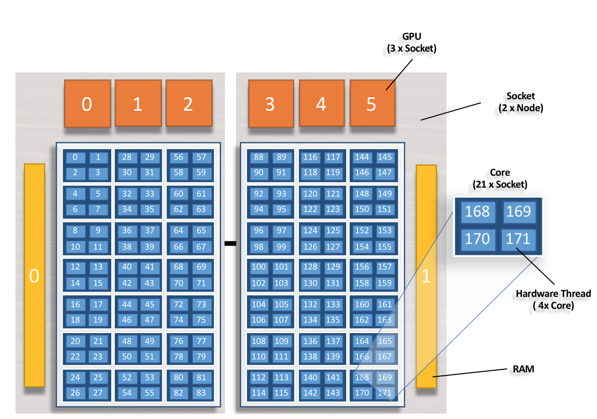
1 node
2 sockets (grey)
42 physical cores* (dark blue)
168 hardware cores (light blue)
6 GPUs (orange)
2 Memory blocks (yellow)
*Core Isolation: 1 core on each socket has been set aside for overhead and is not available for allocation through jsrun. The core has been omitted and is not shown in the above image.
Resource Sets
While jsrun performs similar job launching functions as aprun and
mpirun, its syntax is very different. A large reason for syntax
differences is the introduction of the resource set concept. Through
resource sets, jsrun can control how a node appears to each job. Users
can, through jsrun command line flags, control which resources on a node
are visible to a job. Resource sets also allow the ability to run
multiple jsruns simultaneously within a node. Under the covers, a
resource set is a cgroup.
At a high level, a resource set allows users to configure what a node look like to their job.
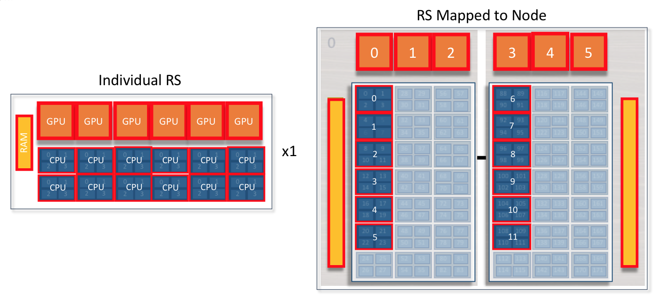
jsrun will create one or more resource sets within a node. Each resource set will contain 1 or more cores and 0 or more GPUs. A resource set can span sockets, but it may not span a node. While a resource set can span sockets within a node, consideration should be given to the cost of cross-socket communication. By creating resource sets only within sockets, costly communication between sockets can be prevented.
Subdividing a Node with Resource Sets
Resource sets provides the ability to subdivide node’s resources into smaller groups. The following examples show how a node can be subdivided and how many resource set could fit on a node.
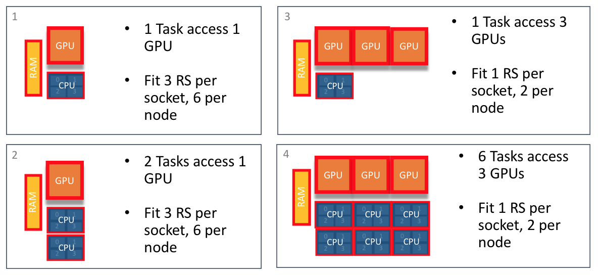
Multiple Methods to Creating Resource Sets
Resource sets should be created to fit code requirements. The following examples show multiple ways to create resource sets that allow two MPI tasks access to a single GPU.
6 resource sets per node: 1 GPU, 2 cores per (Titan)

In this case, CPUs can only see single assigned GPU.
2 resource sets per node: 3 GPUs and 6 cores per socket
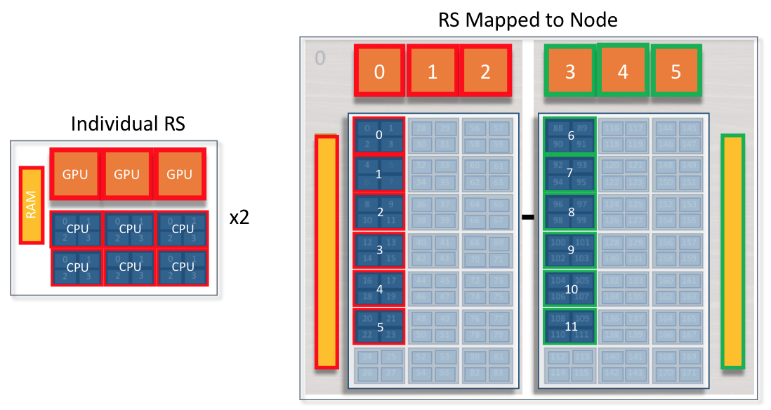
In this case, all 6 CPUs can see 3 GPUs. Code must manage CPU -> GPU communication. CPUs on socket0 can not access GPUs or Memory on socket1.
Single resource set per node: 6 GPUs, 12 cores
In this case, all 12 CPUs can see all node’s 6 GPUs. Code must manage CPU to GPU communication. CPUs on socket0 can access GPUs and Memory on socket1. Code must manage cross socket communication.
Designing a Resource Set
Resource sets allow each jsrun to control how the node appears to a code. This method is unique to jsrun, and requires thinking of each job launch differently than aprun or mpirun. While the method is unique, the method is not complicated and can be reasoned in a few basic steps.
The first step to creating resource sets is understanding how a code would like the node to appear. For example, the number of tasks/threads per GPU. Once this is understood, the next step is to simply calculate the number of resource sets that can fit on a node. From here, the number of needed nodes can be calculated and passed to the batch job request.
The basic steps to creating resource sets:
- Understand how your code expects to interact with the system.
How many tasks/threads per GPU?
Does each task expect to see a single GPU? Do multiple tasks expect to share a GPU? Is the code written to internally manage task to GPU workload based on the number of available cores and GPUs?
- Create resource sets containing the needed GPU to task binding
Based on how your code expects to interact with the system, you can create resource sets containing the needed GPU and core resources. If a code expects to utilize one GPU per task, a resource set would contain one core and one GPU. If a code expects to pass work to a single GPU from two tasks, a resource set would contain two cores and one GPU.
- Decide on the number of resource sets needed
Once you understand tasks, threads, and GPUs in a resource set, you simply need to decide the number of resource sets needed.
As on any system, it is useful to keep in mind the hardware underneath every execution. This is particularly true when laying out resource sets.
Launching a Job with jsrun
jsrun Format
jsrun [ -n #resource sets ] [tasks, threads, and GPUs within each resource set] program [ program args ]
Common jsrun Options
Below are common jsrun options. More flags and details can be found in the jsrun man page. The defaults listed in the table below are the OLCF defaults and take precedence over those mentioned in the man page.
Flags |
Description |
Default Value |
|
|---|---|---|---|
Long |
Short |
||
|
|
Number of resource sets |
All available physical cores |
|
|
Number of MPI tasks (ranks) per resource set |
Not set by default, instead total tasks (-p) set |
|
|
Number of CPUs (cores) per resource set. |
1 |
|
|
Number of GPUs per resource set |
0 |
|
|
Binding of tasks within a resource set. Can be none, rs, or packed:# |
packed:1 |
|
|
Number of resource sets per host |
No default |
|
|
Latency Priority. Controls layout priorities. Can currently be cpu-cpu or gpu-cpu |
gpu-cpu,cpu-mem,cpu-cpu |
|
|
How tasks are started on resource sets |
packed |
It’s recommended to explicitly specify jsrun options and not rely on the
default values. This most often includes --nrs,--cpu_per_rs,
--gpu_per_rs, --tasks_per_rs, --bind, and --launch_distribution.
Jsrun Examples
The below examples were launched in the following 2 node interactive batch job:
summit> bsub -nnodes 2 -Pprj123 -W02:00 -Is $SHELL
Single MPI Task, single GPU per RS
The following example will create 12 resource sets each with 1 MPI task and 1 GPU. Each MPI task will have access to a single GPU.
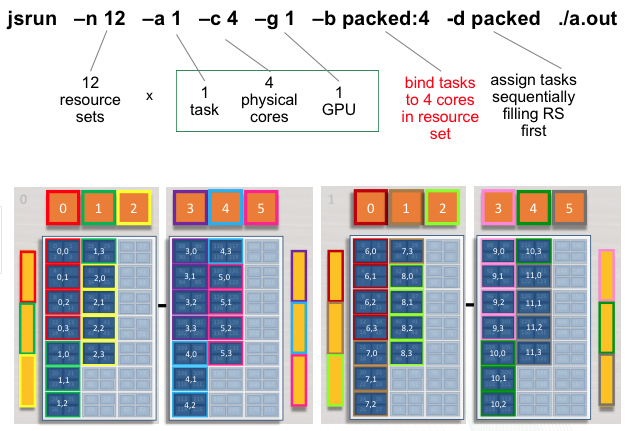
Rank 0 will have access to GPU 0 on the first node ( red resource set). Rank 1 will have access to GPU 1 on the first node ( green resource set). This pattern will continue until 12 resources sets have been created.
The following jsrun command will request 12 resource sets (-n12) 6
per node (-r6). Each resource set will contain 1 MPI task (-a1),
1 GPU (-g1), and 1 core (-c1).
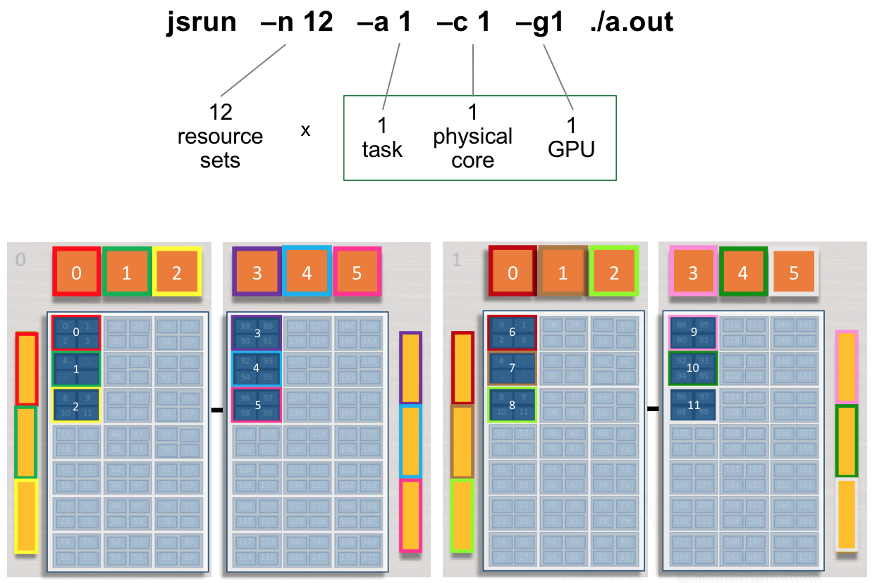
summit> jsrun -n12 -r6 -a1 -g1 -c1 ./a.out
Rank:    0; NumRanks: 12; RankCore:   0; Hostname: h41n04; GPU: 0
Rank:    1; NumRanks: 12; RankCore:   4; Hostname: h41n04; GPU: 1
Rank:    2; NumRanks: 12; RankCore:   8; Hostname: h41n04; GPU: 2
Rank:    3; NumRanks: 12; RankCore:  88; Hostname: h41n04; GPU: 3
Rank:    4; NumRanks: 12; RankCore:  92; Hostname: h41n04; GPU: 4
Rank:    5; NumRanks: 12; RankCore:  96; Hostname: h41n04; GPU: 5

Rank:    6; NumRanks: 12; RankCore:   0; Hostname: h41n03; GPU: 0
Rank:    7; NumRanks: 12; RankCore:   4; Hostname: h41n03; GPU: 1
Rank:    8; NumRanks: 12; RankCore:   8; Hostname: h41n03; GPU: 2
Rank:    9; NumRanks: 12; RankCore:  88; Hostname: h41n03; GPU: 3
Rank:   10; NumRanks: 12; RankCore:  92; Hostname: h41n03; GPU: 4
Rank:   11; NumRanks: 12; RankCore:  96; Hostname: h41n03; GPU: 5
Multiple tasks, single GPU per RS
The following jsrun command will request 12 resource sets (-n12).
Each resource set will contain 2 MPI tasks (-a2), 1 GPU
(-g1), and 2 cores (-c2). 2 MPI tasks will have access to a
single GPU. Ranks 0 - 1 will have access to GPU 0 on the first node (
red resource set). Ranks 2 - 3 will have access to GPU 1 on the first
node ( green resource set). This pattern will continue until 12 resource
sets have been created.
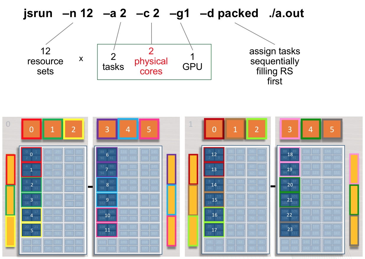
Adding cores to the RS: The -c flag should be used to request
the needed cores for tasks and treads. The default -c core count is 1.
In the above example, if -c is not specified both tasks will run on a
single core.
summit> jsrun -n12 -a2 -g1 -c2 -dpacked ./a.out | sort
Rank:    0; NumRanks: 24; RankCore:   0; Hostname: a01n05; GPU: 0
Rank:    1; NumRanks: 24; RankCore:   4; Hostname: a01n05; GPU: 0

Rank:    2; NumRanks: 24; RankCore:   8; Hostname: a01n05; GPU: 1
Rank:    3; NumRanks: 24; RankCore:  12; Hostname: a01n05; GPU: 1

Rank:    4; NumRanks: 24; RankCore:  16; Hostname: a01n05; GPU: 2
Rank:    5; NumRanks: 24; RankCore:  20; Hostname: a01n05; GPU: 2

Rank:    6; NumRanks: 24; RankCore:  88; Hostname: a01n05; GPU: 3
Rank:    7; NumRanks: 24; RankCore:  92; Hostname: a01n05; GPU: 3

Rank:    8; NumRanks: 24; RankCore:  96; Hostname: a01n05; GPU: 4
Rank:    9; NumRanks: 24; RankCore: 100; Hostname: a01n05; GPU: 4

Rank:   10; NumRanks: 24; RankCore: 104; Hostname: a01n05; GPU: 5
Rank:   11; NumRanks: 24; RankCore: 108; Hostname: a01n05; GPU: 5

Rank:   12; NumRanks: 24; RankCore:   0; Hostname: a01n01; GPU: 0
Rank:   13; NumRanks: 24; RankCore:   4; Hostname: a01n01; GPU: 0

Rank:   14; NumRanks: 24; RankCore:   8; Hostname: a01n01; GPU: 1
Rank:   15; NumRanks: 24; RankCore:  12; Hostname: a01n01; GPU: 1

Rank:   16; NumRanks: 24; RankCore:  16; Hostname: a01n01; GPU: 2
Rank:   17; NumRanks: 24; RankCore:  20; Hostname: a01n01; GPU: 2

Rank:   18; NumRanks: 24; RankCore:  88; Hostname: a01n01; GPU: 3
Rank:   19; NumRanks: 24; RankCore:  92; Hostname: a01n01; GPU: 3

Rank:   20; NumRanks: 24; RankCore:  96; Hostname: a01n01; GPU: 4
Rank:   21; NumRanks: 24; RankCore: 100; Hostname: a01n01; GPU: 4

Rank:   22; NumRanks: 24; RankCore: 104; Hostname: a01n01; GPU: 5
Rank:   23; NumRanks: 24; RankCore: 108; Hostname: a01n01; GPU: 5

summit>
Multiple Task, Multiple GPU per RS
The following example will create 4 resource sets each with 6 tasks and
3 GPUs. Each set of 6 MPI tasks will have access to 3 GPUs. Ranks 0 - 5
will have access to GPUs 0 - 2 on the first socket of the first node (
red resource set). Ranks 6 - 11 will have access to GPUs 3 - 5 on the
second socket of the first node ( green resource set). This pattern will
continue until 4 resource sets have been created. The following jsrun
command will request 4 resource sets (-n4). Each resource set will
contain 6 MPI tasks (-a6), 3 GPUs (-g3), and 6 cores
(-c6).
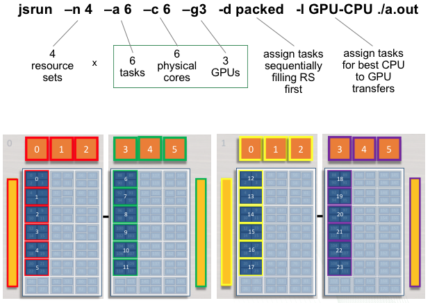
summit> jsrun -n 4 -a 6 -c 6 -g 3 -d packed -l GPU-CPU ./a.out
Rank:    0; NumRanks: 24; RankCore:   0; Hostname: a33n06; GPU: 0, 1, 2
Rank:    1; NumRanks: 24; RankCore:   4; Hostname: a33n06; GPU: 0, 1, 2
Rank:    2; NumRanks: 24; RankCore:   8; Hostname: a33n06; GPU: 0, 1, 2
Rank:    3; NumRanks: 24; RankCore:  12; Hostname: a33n06; GPU: 0, 1, 2
Rank:    4; NumRanks: 24; RankCore:  16; Hostname: a33n06; GPU: 0, 1, 2
Rank:    5; NumRanks: 24; RankCore:  20; Hostname: a33n06; GPU: 0, 1, 2

Rank:    6; NumRanks: 24; RankCore:  88; Hostname: a33n06; GPU: 3, 4, 5
Rank:    7; NumRanks: 24; RankCore:  92; Hostname: a33n06; GPU: 3, 4, 5
Rank:    8; NumRanks: 24; RankCore:  96; Hostname: a33n06; GPU: 3, 4, 5
Rank:    9; NumRanks: 24; RankCore: 100; Hostname: a33n06; GPU: 3, 4, 5
Rank:   10; NumRanks: 24; RankCore: 104; Hostname: a33n06; GPU: 3, 4, 5
Rank:   11; NumRanks: 24; RankCore: 108; Hostname: a33n06; GPU: 3, 4, 5

Rank:   12; NumRanks: 24; RankCore:   0; Hostname: a33n05; GPU: 0, 1, 2
Rank:   13; NumRanks: 24; RankCore:   4; Hostname: a33n05; GPU: 0, 1, 2
Rank:   14; NumRanks: 24; RankCore:   8; Hostname: a33n05; GPU: 0, 1, 2
Rank:   15; NumRanks: 24; RankCore:  12; Hostname: a33n05; GPU: 0, 1, 2
Rank:   16; NumRanks: 24; RankCore:  16; Hostname: a33n05; GPU: 0, 1, 2
Rank:   17; NumRanks: 24; RankCore:  20; Hostname: a33n05; GPU: 0, 1, 2

Rank:   18; NumRanks: 24; RankCore:  88; Hostname: a33n05; GPU: 3, 4, 5
Rank:   19; NumRanks: 24; RankCore:  92; Hostname: a33n05; GPU: 3, 4, 5
Rank:   20; NumRanks: 24; RankCore:  96; Hostname: a33n05; GPU: 3, 4, 5
Rank:   21; NumRanks: 24; RankCore: 100; Hostname: a33n05; GPU: 3, 4, 5
Rank:   22; NumRanks: 24; RankCore: 104; Hostname: a33n05; GPU: 3, 4, 5
Rank:   23; NumRanks: 24; RankCore: 108; Hostname: a33n05; GPU: 3, 4, 5
summit>
Common Use Cases
The following table provides a quick reference for creating resource
sets of various common use cases. The -n flag can be altered to
specify the number of resource sets needed.
Resource Sets |
MPI Tasks |
Threads |
Physical Cores |
GPUs |
jsrun Command |
|---|---|---|---|---|---|
1 |
42 |
0 |
42 |
0 |
jsrun -n1 -a42 -c42 -g0 |
1 |
1 |
0 |
1 |
1 |
jsrun -n1 -a1 -c1 -g1 |
1 |
2 |
0 |
2 |
1 |
jsrun -n1 -a2 -c2 -g1 |
1 |
1 |
0 |
1 |
2 |
jsrun -n1 -a1 -c1 -g2 |
1 |
1 |
21 |
21 |
3 |
jsrun -n1 -a1 -c21 -g3 -bpacked:21 |
jsrun Tools
This section describes tools that users might find helpful to better understand the jsrun job launcher.
hello_jsrun
hello_jsrun is a “Hello World”-type program that users can run on Summit nodes to better understand how MPI ranks and OpenMP threads are mapped to the hardware. https://code.ornl.gov/t4p/Hello_jsrun A screencast showing how to use Hello_jsrun is also available: https://vimeo.com/261038849
Job Step Viewer
Job Step Viewer provides a graphical view of an application’s runtime layout on Summit.
It allows users to preview and quickly iterate with multiple jsrun options to
understand and optimize job launch.
For bug reports or suggestions, please email help@olcf.ornl.gov.
Usage
- Request a Summit allocation
bsub -W 10 -nnodes 2 -P $OLCF_PROJECT_ID -Is $SHELL
- Load the
job-step-viewermodule module load job-step-viewer
- Load the
- Test out a
jsrunline by itself, or provide an executable as normal jsrun -n12 -r6 -c7 -g1 -a1 -EOMP_NUM_THREADS=7 -brs
- Test out a
- Visit the provided URL
Note
Most Terminal applications have built-in shortcuts to directly open web addresses in the default browser.
MacOS Terminal.app: hold Command (⌘) and double-click on the URL
iTerm2: hold Command (⌘) and single-click on the URL
Limitations
(currently) Compiled with GCC toolchain only
Does not support MPMD-mode via ERF
OpenMP only supported with use of the
OMP_NUM_THREADSenvironment variable.
More Information
This section provides some of the most commonly used LSF commands as
well as some of the most useful options to those commands and
information on jsrun, Summit’s job launch command. Many commands
have much more information than can be easily presented here. More
information about these commands is available via the online manual
(i.e. man jsrun). Additional LSF information can be found on IBM’s
website.
Using Multithreading in a Job
Hardware Threads: Multiple Threads per Core
Each physical core on Summit contains 4 hardware threads. The SMT level can be set using LSF flags (the default is smt4):
SMT1
#BSUB -alloc_flags smt1
jsrun -n1 -c1 -a1 -bpacked:1 csh -c 'echo $OMP_PLACES’
0
SMT2
#BSUB -alloc_flags smt2
jsrun -n1 -c1 -a1 -bpacked:1 csh -c 'echo $OMP_PLACES’
{0:2}
SMT4
#BSUB -alloc_flags smt4
jsrun -n1 -c1 -a1 -bpacked:1 csh -c 'echo $OMP_PLACES’
{0:4}
Controlling Number of Threads for Tasks
In addition to specifying the SMT level, you can also control the
number of threads per MPI task by exporting the OMP_NUM_THREADS
environment variable. If you don’t export it yourself, Jsrun will
automatically set the number of threads based on the number of cores
requested (-c) and the binding (-b) option. It is better to be
explicit and set the OMP_NUM_THREADS value yourself rather than
relying on Jsrun constructing it for you. Especially when you are
using Job Step Viewer which relies on the presence of that
environment variable to give you visual thread assignment information.
In the below example, you could also do export OMP_NUM_THREADS=16 in your
job script instead of passing it as a -E flag to jsrun. The below example
starts 1 resource set with 2 tasks and 8 cores, 4 cores bound to each task,
16 threads for each task. We can set 16 threads since there are 4 cores
per task and the default is smt4 for each core (4 * 4 = 16 threads).
jsrun -n1 -a2 -c8 -g1 -bpacked:4 -dpacked -EOMP_NUM_THREADS=16 csh -c 'echo $OMP_NUM_THREADS $OMP_PLACES'

16 0:4,4:4,8:4,12:4
16 16:4,20:4,24:4,28:4
Be careful with assigning threads to tasks, as you might end up oversubscribing your cores. For example
jsrun -n1 -a2 -c8 -g1 -bpacked:4 -dpacked -EOMP_NUM_THREADS=32 csh -c 'echo $OMP_NUM_THREADS $OMP_PLACES'

Warning: OMP_NUM_THREADS=32 is greater than available PU's
Warning: OMP_NUM_THREADS=32 is greater than available PU's
Warning: OMP_NUM_THREADS=32 is greater than available PU's
Warning: OMP_NUM_THREADS=32 is greater than available PU's
32 16:4,20:4,24:4,28:4
32 0:4,4:4,8:4,12:4
You can use hello_jsrun or Job Step Viewer to see how the cores are being oversubscribed.
Because of how jsrun sets up OMP_NUM_THREADS based on -c and
-b options if you don’t specify the environment variable yourself,
you can accidentally end up oversubscribing your cores. For example
jsrun -n1 -a2 -c8 -g1 -brs -dpacked  csh -c 'echo $OMP_NUM_THREADS $OMP_PLACES'

Warning: more than 1 task/rank assigned to a core
Warning: more than 1 task/rank assigned to a core
32 0:4,4:4,8:4,12:4,16:4,20:4,24:4,28:4
32 0:4,4:4,8:4,12:4,16:4,20:4,24:4,28:4
Because jsrun sees 8 cores and the -brs flag, it assigns all 8 cores to
each of the 2 tasks in the resource set. Jsrun will set up OMP_NUM_THREADS
as 32 (8 cores with 4 threads per core) which will apply to all the
tasks in the resource set. This means that each task sees that it can
have 32 threads (which means 64 threads for the 2 tasks combined) which
will oversubscribe the cores and may decrease efficiency as a result.
Example: Single Task, Single GPU, Multiple Threads per RS
The following example will create 12 resource sets each with 1 task, 4
threads, and 1 GPU. Each MPI task will start 4 threads and have access
to 1 GPU. Rank 0 will have access to GPU 0 and start 4 threads on the
first socket of the first node ( red resource set). Rank 2 will have
access to GPU 1 and start 4 threads on the second socket of the first
node ( green resource set). This pattern will continue until 12 resource
sets have been created. The following jsrun command will create 12
resource sets (-n12). Each resource set will contain 1 MPI task
(-a1), 1 GPU (-g1), and 4 cores (-c4). Notice that
more cores are requested than MPI tasks; the extra cores will be needed
to place threads. Without requesting additional cores, threads will be
placed on a single core.
Requesting Cores for Threads: The -c flag should be used to
request additional cores for thread placement. Without requesting
additional cores, threads will be placed on a single core.
Binding Cores to Tasks: The -b binding flag should be used to
bind cores to tasks. Without specifying binding, all threads will be
bound to the first core.
summit> setenv OMP_NUM_THREADS 4
summit> jsrun -n12 -a1 -c4 -g1 -b packed:4 -d packed ./a.out
Rank: 0; RankCore: 0; Thread: 0; ThreadCore: 0; Hostname: a33n06; OMP_NUM_PLACES: {0},{4},{8},{12}
Rank: 0; RankCore: 0; Thread: 1; ThreadCore: 4; Hostname: a33n06; OMP_NUM_PLACES: {0},{4},{8},{12}
Rank: 0; RankCore: 0; Thread: 2; ThreadCore: 8; Hostname: a33n06; OMP_NUM_PLACES: {0},{4},{8},{12}
Rank: 0; RankCore: 0; Thread: 3; ThreadCore: 12; Hostname: a33n06; OMP_NUM_PLACES: {0},{4},{8},{12}

Rank: 1; RankCore: 16; Thread: 0; ThreadCore: 16; Hostname: a33n06; OMP_NUM_PLACES: {16},{20},{24},{28}
Rank: 1; RankCore: 16; Thread: 1; ThreadCore: 20; Hostname: a33n06; OMP_NUM_PLACES: {16},{20},{24},{28}
Rank: 1; RankCore: 16; Thread: 2; ThreadCore: 24; Hostname: a33n06; OMP_NUM_PLACES: {16},{20},{24},{28}
Rank: 1; RankCore: 16; Thread: 3; ThreadCore: 28; Hostname: a33n06; OMP_NUM_PLACES: {16},{20},{24},{28}

...

Rank: 10; RankCore: 104; Thread: 0; ThreadCore: 104; Hostname: a33n05; OMP_NUM_PLACES: {104},{108},{112},{116}
Rank: 10; RankCore: 104; Thread: 1; ThreadCore: 108; Hostname: a33n05; OMP_NUM_PLACES: {104},{108},{112},{116}
Rank: 10; RankCore: 104; Thread: 2; ThreadCore: 112; Hostname: a33n05; OMP_NUM_PLACES: {104},{108},{112},{116}
Rank: 10; RankCore: 104; Thread: 3; ThreadCore: 116; Hostname: a33n05; OMP_NUM_PLACES: {104},{108},{112},{116}

Rank: 11; RankCore: 120; Thread: 0; ThreadCore: 120; Hostname: a33n05; OMP_NUM_PLACES: {120},{124},{128},{132}
Rank: 11; RankCore: 120; Thread: 1; ThreadCore: 124; Hostname: a33n05; OMP_NUM_PLACES: {120},{124},{128},{132}
Rank: 11; RankCore: 120; Thread: 2; ThreadCore: 128; Hostname: a33n05; OMP_NUM_PLACES: {120},{124},{128},{132}
Rank: 11; RankCore: 120; Thread: 3; ThreadCore: 132; Hostname: a33n05; OMP_NUM_PLACES: {120},{124},{128},{132}

summit>
Launching Multiple Jsruns
Jsrun provides the ability to launch multiple jsrun job launches within a
single batch job allocation. This can be done within a single node, or across
multiple nodes.
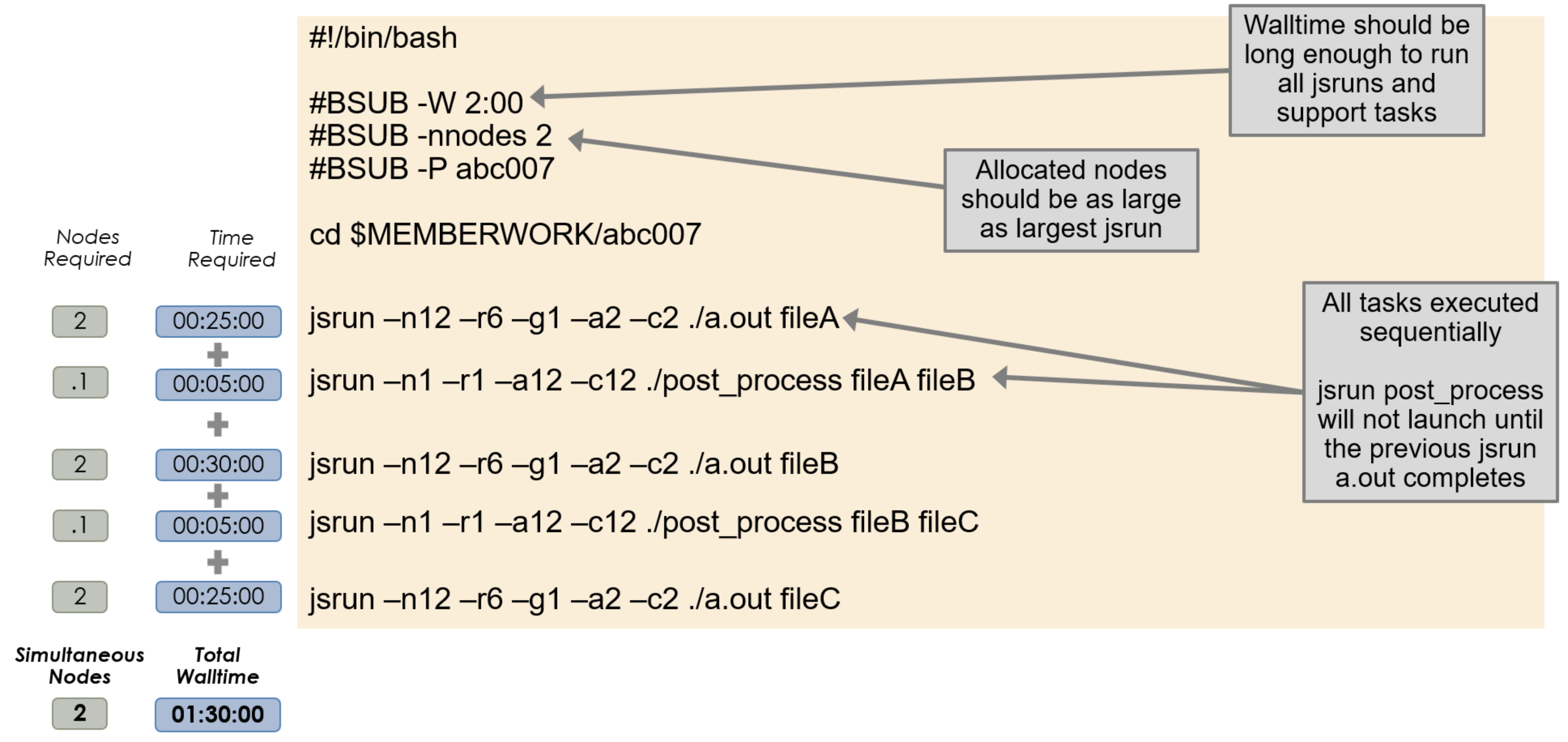
Sequential Job Steps
By default, multiple invocations of jsrun in a job script will execute
serially in order. In this configuration, jobs will launch one at a time and
the next one will not start until the previous is complete. The batch node
allocation is equal to the largest jsrun submitted, and the total walltime
must be equal to or greater then the sum of all jsruns issued.
Simultaneous Job Steps
To execute multiple job steps concurrently, standard UNIX process
backgrounding can be used by adding a & at the end of the command. This
will return control to the job script and execute the next command immediately,
allowing multiple job launches to start at the same time. The jsruns will not
share core/gpu resources in this configuration. The batch node allocation is
equal to the sum of those of each jsrun, and the total walltime must be equal
to or greater than that of the longest running jsrun task.
A wait command must follow all backgrounded processes to prevent the job
from appearing completed and exiting prematurely.
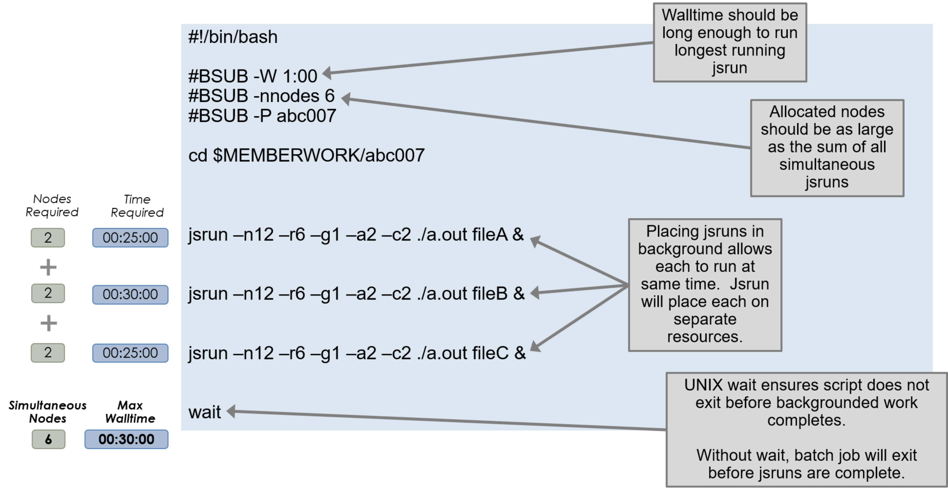
The following example executes three backgrounded job steps and waits for them to finish before the job ends.
#!/bin/bash
#BSUB -P ABC123
#BSUB -W 3:00
#BSUB -nnodes 1
#BSUB -J RunSim123
#BSUB -o RunSim123.%J
#BSUB -e RunSim123.%J

cd $MEMBERWORK/abc123
jsrun <options> ./a.out &
jsrun <options> ./a.out &
jsrun <options> ./a.out &
wait
As submission scripts (and interactive sessions) are executed on batch nodes, the number of concurrent job steps is limited by the per-user process limit on a batch node, where a single user is only permitted 4096 simultaneous processes. This limit is per user on each batch node, not per batch job.
Each job step will create 3 processes, and JSM management may create up to ~23 processes. This creates an upper-limit of ~1350 simultaneous job steps.
If JSM or PMIX errors occur as the result of backgrounding many job steps, using the
--immediate option to jsrun may help, as shown in the following example.
#!/bin/bash
#BSUB -P ABC123
#BSUB -W 3:00
#BSUB -nnodes 1
#BSUB -J RunSim123
#BSUB -o RunSim123.%J
#BSUB -e RunSim123.%J

cd $MEMBERWORK/abc123
jsrun <options> --immediate ./a.out
jsrun <options> --immediate ./a.out
jsrun <options> --immediate ./a.out
Note
By default, jsrun --immediate does not produce stdout or
stderr. To capture stdout and/or stderr when using this option,
additionally include --stdio_stdout/-o and/or
--stdio_stderr/-k.
Using jslist
To view the status of multiple jobs launched sequentially or concurrently within a batch script, you can use jslist to see which are completed, running, or still queued. If you are using it outside of an interactive batch job, use the -c option to specify the CSM allocation ID number. The following example shows how to obtain the CSM allocation number for a non interactive job and then check its status.
$ bsub test.lsf
Job <26238> is submitted to default queue <batch>.

$ bjobs -l 26238 | grep CSM_ALLOCATION_ID
Sun Feb 16 19:01:18: CSM_ALLOCATION_ID=34435

$ jslist -c 34435
  parent         cpus     gpus     exit
  ID  ID    nrs  per RS  per RS   status    status
 ===========================================================
   1   0    12     4       1        0       Running
Explicit Resource Files (ERF)
Explicit Resource Files provide even more fine-granied control over how processes are mapped onto compute nodes. ERFs can define job step options such as rank placement/binding, SMT/CPU/GPU resources, compute hosts, among many others. If you find that the most common jsrun options do not readily provide the resource layout you need, we recommend considering ERF files.
A common source of confusion when using ERFs is how physical cores are
enumerated. See the tutorial on ERF CPU
Indexing for a
discussion of the cpu_index_using control and its interaction with various
SMT modes.
Note
Please note, a known bug is currently preventing execution of most ERF use cases. We are working to resolve the issue.
CUDA-Aware MPI
CUDA-aware MPI and GPUDirect are often used interchangeably, but they are distinct topics.
CUDA-aware MPI allows GPU buffers (e.g., GPU memory allocated with
cudaMalloc) to be used directly in MPI calls rather than requiring
data to be manually transferred to/from a CPU buffer (e.g., using
cudaMemcpy) before/after passing data in MPI calls. By itself,
CUDA-aware MPI does not specify whether data is staged through
CPU memory or, for example, transferred directly between GPUs when
passing GPU buffers to MPI calls. That is where GPUDirect comes in.
GPUDirect is a technology that can be implemented on a system to enhance
CUDA-aware MPI by allowing data transfers directly between GPUs on the
same node (peer-to-peer) and/or directly between GPUs on different nodes
(with RDMA support) without the need to stage data through CPU memory.
On Summit, both peer-to-peer and RDMA support are implemented. To enable
CUDA-aware MPI in a job, use the following argument to jsrun:
jsrun --smpiargs="-gpu" ...
Not using the --smpiargs="-gpu" flag might result in confusing segmentation
faults. If you see a segmentation fault when trying to do GPU aware MPI, check to
see if you have the flag set correctly.
Monitoring Jobs
LSF provides several utilities with which you can monitor jobs. These include monitoring the queue, getting details about a particular job, viewing STDOUT/STDERR of running jobs, and more.
The most straightforward monitoring is with the bjobs command. This
command will show the current queue, including both pending and running
jobs. Running bjobs -l will provide much more detail about a job (or
group of jobs). For detailed output of a single job, specify the job id
after the -l. For example, for detailed output of job 12345, you can
run bjobs -l 12345 . Other options to bjobs are shown below. In
general, if the command is specified with -u all it will show
information for all users/all jobs. Without that option, it only shows
your jobs. Note that this is not an exhaustive list. See man bjobs
for more information.
Command |
Description |
|---|---|
|
Show your current jobs in the queue |
|
Show currently queued jobs for all users |
|
Shows currently-queued jobs for project ABC123 |
|
Don’t format output (might be useful if you’re using the output in a script) |
|
Show jobs in all states, including recently finished jobs |
|
Show long/detailed output |
|
Show long/detailed output for jobs 12345 |
|
Show details for recently completed jobs |
|
Show suspended jobs, including the reason(s) they’re suspended |
|
Show running jobs |
|
Show pending jobs |
|
Use “wide” formatting for output |
If you want to check the STDOUT/STDERR of a currently running job, you
can do so with the bpeek command. The command supports several
options:
Command |
Description |
|---|---|
|
Show STDOUT/STDERR for the job you’ve most recently submitted with the name jobname |
|
Show STDOUT/STDERR for job 12345 |
|
Used with other options. Makes |
The OLCF also provides jobstat, which adds dividers in the queue to
identify jobs as running, eligible, or blocked. Run without arguments,
jobstat provides a snapshot of the entire batch queue. Additional
information, including the number of jobs in each state, total nodes
available, and relative job priority are also included.
jobstat -u <username> restricts output to only the jobs of a
specific user. See the jobstat man page for a full list of
formatting arguments.
$ jobstat -u <user>
--------------------------- Running Jobs: 2 (4544 of 4604 nodes, 98.70%) ---------------------------
JobId    Username   Project          Nodes Remain     StartTime       JobName
331590   user     project           2     57:06      04/09 10:06:23  Not_Specified
331707   user     project           40    39:47      04/09 11:04:04  runA
----------------------------------------- Eligible Jobs: 3 -----------------------------------------
JobId    Username   Project          Nodes Walltime   QueueTime       Priority JobName
331712   user     project           80    45:00      04/09 11:06:23  501.00   runB
331713   user     project           90    45:00      04/09 11:07:19  501.00   runC
331714   user     project           100   45:00      04/09 11:07:49  501.00   runD
----------------------------------------- Blocked Jobs: 1 ------------------------------------------
JobId    Username   Project          Nodes Walltime   BlockReason
331715   user        project           12    2:00:00    Job dependency condition not satisfied
Inspecting Backfill
bjobs and jobstat help to identify what’s currently running and
scheduled to run, but sometimes it’s beneficial to know how much of the
system is not currently in use or scheduled for use.
The bslots command can be used to inspect backfill windows and answer
the question “How many nodes are currently available, and for how long
will they remain available?” This can be thought of as identifying gaps in
the system’s current job schedule. By intentionally requesting resources
within the parameters of a backfill window, one can potentially shorten
their queued time and improve overall system utilization.
LSF uses “slots” to describe allocatable resources. Summit compute nodes have 1
slot per CPU core, for a total of 42 per node ([2x] Power9 CPUs, each
with 21 cores). Since Summit nodes are scheduled in whole-node
allocations, the output from bslots can be divided by 42 to see how
many nodes are currently available.
By default, bslots output includes launch node slots, which can
cause unwanted and inflated fractional node values. The output can
be adjusted to reflect only available compute node slots with the
flag -R”select[CN]”. For example,
$ bslots -R"select[CN]"
SLOTS          RUNTIME
42             25 hours 42 minutes 51 seconds
27384          1 hours 11 minutes 50 seconds
27384 compute node slots / 42 slots per node = 652 compute nodes are available for 1 hour, 11 minutes, 50 seconds.
A more specific bslots query could check for a backfill window with
space to fit a 1000 node job for 10 minutes:
$ bslots -R"select[CN]" -n $((1000*42)) -W10
SLOTS          RUNTIME
127764         22 minutes 55 seconds
There is no guarantee that the slots reported by bslots will still
be available at time of new job submission.
Interacting With Jobs
Sometimes it’s necessary to interact with a batch job after it has been submitted. LSF provides several commands for interacting with already-submitted jobs.
Many of these commands can operate on either one job or a group of jobs. In general, they only operate on the most recently submitted job that matches other criteria provided unless “0” is specified as the job id.
Suspending and Resuming Jobs
LSF supports user-level suspension and resumption of jobs. Jobs are
suspended with the bstop command and resumed with the bresume
command. The simplest way to invoke these commands is to list the job id
to be suspended/resumed:
bstop 12345
bresume 12345
Instead of specifying a job id, you can specify other criteria that will
allow you to suspend some/all jobs that meet other criteria such as a
job name, a queue name, etc. These are described in the manpages for
bstop and bresume.
Signaling Jobs
You can send signals to jobs with the bkill command. While the
command name suggests its only purpose is to terminate jobs, this is not
the case. Similar to the kill command found in Unix-like operating
systems, this command can be used to send various signals (not just
SIGTERM and SIGKILL) to jobs. The command can accept both
numbers and names for signals. For a list of accepted signal names, run
bkill -l. Common ways to invoke the command include:
Command |
Description |
|---|---|
|
Force a job to stop by sending |
|
Send |
|
Send signal 9 to job 12345 |
Like bstop and bresume, bkill command also supports
identifying the job(s) to be signaled by criteria other than the job id.
These include some/all jobs with a given name, in a particular queue,
etc. See man bkill for more information.
Checkpointing Jobs
LSF documentation mentions the bchkpnt and brestart commands for
checkpointing and restarting jobs, as well as the -k option to
bsub for configuring checkpointing. Since checkpointing is very
application specific and a wide range of applications run on OLCF
resources, this type of checkpointing is not configured on Summit. If
you wish to use checkpointing (which is highly encouraged), you’ll need
to configure it within your application.
If you wish to implement some form of on-demand checkpointing, keep in mind
the bkill command is really a signaling command and you can have your
job script/application checkpoint as a response to certain signals (such
as SIGUSR1).
Other LSF Commands
The table below summarizes some additional LSF commands that might be useful.
Command |
Description |
|---|---|
|
Show current parameters for LSF. The behavior/available options for some LSF commands depend on settings in various configuration files. This command shows those settings without having to search for the actual files. |
|
Show job dependency information (could be useful in determining what job is keeping another job in a pending state) |
PBS/Torque/MOAB-to-LSF Translation
More details about these commands are given elsewhere in this section; the table below is simply for your convenience in looking up various LSF commands.
Users of other OLCF resources are likely familiar with PBS-like commands which are used by the Torque/Moab instances on other systems. The table below summarizes the equivalent LSF command for various PBS/Torque/Moab commands.
LSF Command |
PBS/Torque/Moab Command |
Description |
|---|---|---|
|
|
Submit the job script job.sh to the batch system |
|
|
Submit an interactive batch job |
|
|
Show jobs currently in the queue NOTE: without the -u all argument, bjobs will only show your jobs |
|
|
Get information about a specific job |
|
|
Get information about completed jobs |
|
|
Get information about pending jobs |
|
|
Get information about running jobs |
|
|
Send a signal to a job |
|
|
Terminate/Kill a job |
|
|
Hold a job/stop a job from running |
|
|
Release a held job |
|
|
Get information about queues |
|
|
Get information about job dependencies |
The table below shows shows LSF (bsub) command-line/batch script options and the PBS/Torque/Moab (qsub) options that provide similar functionality.
LSF Option |
PBS/Torque/Moab Option |
Description |
|---|---|---|
|
|
Request a walltime of 1 hour |
|
|
Request 1024 nodes |
|
|
Charge the job to project ABC123 |
|
No equivalent (set via environment variable) |
Enable multiple MPI tasks to simultaneously access a GPU |
Easy Mode vs. Expert Mode
The Cluster System Management (CSM) component of the job launch environment supports two methods of job submission, termed “easy” mode and “expert” mode. The difference in the modes is where the responsibility for creating the LSF resource string is placed.
In easy mode, the system software converts options such as -nnodes in
a batch script into the resource string needed by the scheduling system.
In expert mode, the user is responsible for creating this string and
options such as -nnodes cannot be used. In easy mode, you will not be
able to use bsub -R to create resource strings. The system will
automatically create the resource string based on your other bsub
options. In expert mode, you will be able to use -R, but you will
not be able to use the following options to bsub: -ln_slots,
-ln_mem, -cn_cu, or -nnodes.
Most users will want to use easy mode. However, if you need precise
control over your job’s resources, such as placement on (or avoidance
of) specific nodes, you will need to use expert mode. To use expert
mode, add #BSUB -csm y to your batch script (or -csm y to
your bsub command line).
System Service Core Isolation
One core per socket is set aside for system service tasks. The cores are not available to jsrun. When listing available resources through jsrun, you will not see cores with hyperthreads 84-87 and 172-175. Isolating a socket’s system services to a single core helps to reduce jitter and improve performance of tasks performed on the socket’s remaining cores.
The isolated core always operates at SMT4 regardless of the batch job’s SMT level.
GPFS System Service Isolation
By default, GPFS system service tasks are forced onto only the isolated
cores. This can be overridden at the batch job level using the
maximizegpfs argument to LSF’s alloc_flags. For example:
#BSUB -alloc_flags maximizegpfs
The maximizegpfs flag will allow GPFS tasks to utilize any core on the compute node. This may be beneficial because it provides more resources for GPFS service tasks, but it may also cause resource contention for the jsrun compute job.
Job Accounting on Summit
Jobs on Summit are scheduled in full node increments; a node’s cores cannot be allocated to multiple jobs. Because the OLCF charges based on what a job makes unavailable to other users, a job is charged for an entire node even if it uses only one core on a node. To simplify the process, users request and are allocated multiples of entire nodes through LSF.
Allocations on Summit are separate from those on Andes and other OLCF resources.
Node-Hour Calculation
The node-hour charge for each batch job will be calculated as follows:
node-hours = nodes requested * ( batch job endtime - batch job starttime )
Where batch job starttime is the time the job moves into a running state, and batch job endtime is the time the job exits a running state.
A batch job’s usage is calculated solely on requested nodes and the batch job’s start and end time. The number of cores actually used within any particular node within the batch job is not used in the calculation. For example, if a job requests (6) nodes through the batch script, runs for (1) hour, uses only (2) CPU cores per node, the job will still be charged for 6 nodes * 1 hour = 6 node-hours.
Viewing Usage
Utilization is calculated daily using batch jobs which complete between 00:00 and 23:59 of the previous day. For example, if a job moves into a run state on Tuesday and completes Wednesday, the job’s utilization will be recorded Thursday. Only batch jobs which write an end record are used to calculate utilization. Batch jobs which do not write end records due to system failure or other reasons are not used when calculating utilization. Jobs which fail because of run-time errors (e.g. the user’s application causes a segmentation fault) are counted against the allocation.
Each user may view usage for projects on which they are members from the command
line tool showusage and the myOLCF site.
On the Command Line via showusage
The showusage utility can be used to view your usage from January 01
through midnight of the previous day. For example:
$ showusage
  Usage:
                           Project Totals
  Project             Allocation      Usage      Remaining     Usage
  _________________|______________|___________|____________|______________
  abc123           |  20000       |   126.3   |  19873.7   |   1560.80
The -h option will list more usage details.
On the Web via myOLCF
More detailed metrics may be found on each project’s usage section of the myOLCF site. The following information is available for each project:
YTD usage by system, subproject, and project member
Monthly usage by system, subproject, and project member
YTD usage by job size groupings for each system, subproject, and project member
Weekly usage by job size groupings for each system, and subproject
Batch system priorities by project and subproject
Project members
The myOLCF site is provided to aid in the utilization and management of OLCF allocations. See the myOLCF Documentation for more information.
If you have any questions or have a request for additional data, please contact the OLCF User Assistance Center.
Other Notes
Compute nodes are only allocated to one job at a time; they are not shared. This is why users request nodes (instead of some other resource such as cores or GPUs) in batch jobs and is why projects are charged based on the number of nodes allocated multiplied by the amount of time for which they were allocated. Thus, a job using only 1 core on each of its nodes is charged the same as a job using every core and every GPU on each of its nodes.
Debugging
Linaro DDT
Linaro DDT is an advanced debugging tool used for scalar, multi-threaded, and large-scale parallel applications. In addition to traditional debugging features (setting breakpoints, stepping through code, examining variables), DDT also supports attaching to already-running processes and memory debugging. In-depth details of DDT can be found in the Official DDT User Guide, and instructions for how to use it on OLCF systems can be found on the Debugging Software page. DDT is the OLCF’s recommended debugging software for large parallel applications.
One of the most useful features of DDT is its remote debugging feature. This allows you to connect to a debugging session on Frontier from a client running on your workstation. The local client provides much faster interaction than you would have if using the graphical client on Frontier. For guidance in setting up the remote client see the Debugging Software page.
GDB
GDB, the GNU Project Debugger, is a command-line debugger useful for traditional debugging and investigating code crashes. GDB lets you debug programs written in Ada, C, C++, Objective-C, Pascal (and many other languages).
GDB is available on Summit under all compiler families:
module load gdb
To use GDB to debug your application run:
gdb ./path_to_executable
Additional information about GDB usage can befound on the GDB Documentation Page.
Valgrind
Valgrind is an instrumentation framework for building dynamic analysis tools. There are Valgrind tools that can automatically detect many memory management and threading bugs, and profile your programs in detail. You can also use Valgrind to build new tools.
The Valgrind distribution currently includes five production-quality tools: a memory error detector, a thread error detector, a cache and branch-prediction profiler, a call-graph generating cache profiler, and a heap profiler. It also includes two experimental tools: a data race detector, and an instant memory leak detector.
The Valgrind tool suite provides a number of debugging and profiling tools. The most popular is Memcheck, a memory checking tool which can detect many common memory errors such as:
Touching memory you shouldn’t (eg. overrunning heap block boundaries, or reading/writing freed memory).
Using values before they have been initialized.
Incorrect freeing of memory, such as double-freeing heap blocks.
Memory leaks.
Valgrind is available on Summit under all compiler families:
module load valgrind
Additional information about Valgrind usage and OLCF-provided builds can be found on the Valgrind Software Page.
Optimizing and Profiling
Profiling GPU Code with NVIDIA Developer Tools
NVIDIA provides developer tools for profiling any code that runs on NVIDIA GPUs. These are the Nsight suite of developer tools: NVIDIA Nsight Systems for collecting a timeline of your application, and NVIDIA Nsight Compute for collecting detailed performance information about specific GPU kernels.
NVIDIA Nsight Systems
The first step to GPU profiling is collecting a timeline of your application.
(This operation is also sometimes called “tracing,” that is, finding
the start and stop timestamps of all activities that occurred on the GPU
or involved the GPU, such as copying data back and forth.) To do this, we
can collect a timeline using the command-line interface, nsys. To use
this tool, load the nsight-systems module.
summit> module load nsight-systems
For example, we can profile the vectorAdd CUDA sample (the CUDA samples
can be found in $OLCF_CUDA_ROOT/samples if the cuda module is loaded.)
summit> jsrun -n1 -a1 -g1 nsys profile -o vectorAdd --stats=true ./vectorAdd
(Note that even if you do not ask for Nsight Systems to create an output file,
but just ask it to print summary statistics with --stats=true, it will create
a temporary file for storing the profiling data, so you will need to work on a
file system that can be written to from a compute node such as GPFS.)
The profiler will print several sections including information about the CUDA API calls made by the application, as well as any GPU kernels that were launched. Nsight Systems can be used for CUDA C++, CUDA Fortran, OpenACC, OpenMP offload, and other programming models that target NVIDIA GPUs, because under the hood they all ultimately take the same path for generating the binary code that runs on the GPU.
If you add the -o option, as above, the report will be saved to file
with the extension .qdrep. That report file can later be analyzed in
the Nsight Systems UI by selecting File > Open and locating the vectorAdd.qdrep
file on your filesystem. Nsight Systems does not currently have a Power9
version of the UI, so you will need to download the UI for your local system, which is supported on
Windows, Mac, and Linux (x86). Then use scp or some other file transfer
utility for copying the report file from Summit to your local machine.
Nsight Systems can be used for MPI runs with multiple ranks, but it is
not a parallel profiler and cannot combine output from multiple ranks.
Instead, each rank must be profiled and analyzed independently. The file
name should be unique for every rank. Nsight Systems knows how to parse
environment variables with the syntax %q{ENV_VAR}, and since Spectrum
MPI provides an environment variable for every process with its MPI rank,
you can do
summit> jsrun -n6 -a1 -g1 nsys profile -o vectorAdd_%q{OMPI_COMM_WORLD_RANK} ./vectorAdd
Then you will have vectorAdd_0.qdrep through vectorAdd_5.qdrep.
(Of course, in this case each rank does the same thing as this is not
an MPI application, but it works the same way for an MPI code.)
For more details about Nsight Systems, consult the product page and the documentation. If you previously
used nvprof and would like to start using the Nsight Developer Tools,
check out this transition guide.
Also, in March 2020 NVIDIA presented a webinar on Nsight Systems which you
can watch on demand.
NVIDIA Nsight Compute
Individual GPU kernels (the discrete chunks of work that are launched by programming languages such as CUDA and OpenACC) can be profiled in detail with NVIDIA Nsight Compute. The typical workflow is to profile your code with Nsight Systems and identify the major performance bottleneck in your application. If that performance bottleneck is on the CPU, it means more code should be ported to the GPU; or, if that bottleneck is in memory management, such as copying data back and forth between the CPU and GPU, you should look for opportunities to reduce that data motion. But if that bottleneck is a GPU kernel, then Nsight Compute can be used to collect performance counters to understand whether the kernel is running efficiently and if there’s anything you can do to improve.
The Nsight Compute command-line interface, nv-nsight-cu-cli, can be
prefixed to your application to collect a report.
summit> module load nsight-compute
summit> jsrun -n1 -a1 -g1 nv-nsight-cu-cli ./vectorAdd
Similar to Nsight Systems, Nsight Compute will create a temporary report file,
even when -o is not specified.
The most important output to look at is the “GPU Speed of Light” section, which tells you what fraction of peak memory throughput and what fraction of peak compute throughput you achieved. Typically if you have achieved higher than 60% of the peak of either subsystem, your kernel would be considered memory-bound or compute-bound (respectively), and if you have not achieved 60% of either this is often a latency-bound kernel. (A common cause of latency issues is not exposing enough parallelism to saturate the GPU’s compute capacity – peak GPU performance can only be achieved when there is enough work to hide the latency of memory accesses and to keep all compute pipelines busy.)
By default, Nsight Compute will collect this performance data for every kernel
in your application. This will take a long time in a real-world application.
It is recommended that you identify a specific kernel to profile and then use
the -k argument to just profile that kernel. (If you don’t know the name of
your kernel, use nsys to obtain that. The flag will pattern match on any
substring of the kernel name.) You can also use the -s option to skip some
number of kernel calls and the -c option to specify how many invocations of
that kernel you want to profile.
If you want to collect information on just a specific performance measurement,
for example the number of bytes written to DRAM, you can do so with the
--metrics option:
summit> jsrun -n1 -a1 -g1 nv-nsight-cu-cli -k vectorAdd --metrics dram__bytes_write.sum ./vectorAdd
The list of available metrics can be obtained with nv-nsight-cu-cli
--query-metrics. Most metrics have both a base name and suffix. Together
these make up the full metric name to pass to nv-nsight-cu-cli. To list
the full names for a collection of metrics, use --query-metrics-mode suffix
--metrics <metrics list>.
As with Nsight Systems, there is a graphical user interface you can load a
report file into (The GUI is only available for Windows, x86_64 Linux and Mac).
Use the -o flag to create a file (the added report extension will be
.nsight-cuprof-report), copy it to your local system, and use the File >
Open File menu item. If you are using multiple MPI ranks, make sure you name
each one independently. Nsight Compute does not yet support the %q syntax
(this will come in a future release), so your job script will have to do the
naming manually; for example, you can create a simple shell script:
$ cat run.sh
#!/bin/bash

nv-nsight-cu-cli -o vectorAdd_$OMPI_COMM_WORLD_RANK ./vectorAdd
For more details on Nsight Compute, check out the product page and the documentation. If you previously used
nvprof and would like to start using Nsight Compute, check out this transition
guide.
Also, in March 2020 NVIDIA presented a webinar on Nsight Compute which you can watch on
demand.
nvprof and nvvp
Prior to Nsight Systems and Nsight Compute, the NVIDIA command line profiling
tool was nvprof, which provides both tracing and kernel profiling
capabilities. Like with Nsight Systems and Nsight Compute, the profiler data
output can be saved and imported into the NVIDIA Visual Profiler for additional
graphical analysis. nvprof is in maintenance mode now: it still works on
Summit and significant bugs will be fixed, but no new feature development is
occurring on this tool.
To use nvprof, the cuda module must be loaded.
summit> module load cuda
A simple “Hello, World!” run using nvprof can be done by adding
“nvprof” to the jsrun (see: Job Launcher (jsrun))
line in your batch script (see Batch Scripts).
...
jsrun -n1 -a1 -g1 nvprof ./hello_world_gpu
...
Although nvprof doesn’t provide aggregated MPI data, the %h and
%p output file modifiers can be used to create separate output files
for each host and process.
...
jsrun -n1 -a1 -g1 nvprof -o output.%h.%p ./hello_world_gpu
...
There are many various metrics and events that the profiler can capture. For example, to output the number of double-precision FLOPS, you may use the following:
...
jsrun -n1 -a1 -g1 nvprof --metrics flops_dp -o output.%h.%p ./hello_world_gpu
...
To see a list of all available metrics and events, use the following:
summit> nvprof --query-metrics
summit> nvprof --query-events
While using nvprof on the command-line is a quick way to gain
insight into your CUDA application, a full visual profile is often even
more useful. For information on how to view the output of nvprof in
the NVIDIA Visual Profiler, see the NVIDIA
Documentation.
Score-P
The Score-P measurement infrastructure is a highly scalable and easy-to-use tool suite for profiling, event tracing, and online analysis of HPC applications. Score-P supports analyzing C, C++ and Fortran applications that make use of multi-processing (MPI, SHMEM), thread parallelism (OpenMP, PThreads) and accelerators (CUDA, OpenCL, OpenACC) and combinations.
For detailed information about using Score-P on Summit and the builds available, please see the Score-P Software Page.
Vampir
Vampir is a software performance visualizer focused on highly parallel applications. It presents a unified view on an application run including the use of programming paradigms like MPI, OpenMP, PThreads, CUDA, OpenCL and OpenACC. It also incorporates file I/O, hardware performance counters and other performance data sources. Various interactive displays offer detailed insight into the performance behavior of the analyzed application. Vampir’s scalable analysis server and visualization engine enable interactive navigation of large amounts of performance data. Score-P and TAU generate OTF2 trace files for Vampir to visualize.
For detailed information about using Vampir on Summit and the builds available, please see the Vampir Software Page.
HPCToolkit
HPCToolkit is an integrated suite of tools for measurement and analysis of program performance on computers ranging from multicore desktop systems to the nation’s largest supercomputers. HPCToolkit provides accurate measurements of a program’s work, resource consumption, and inefficiency, correlates these metrics with the program’s source code, works with multilingual, fully optimized binaries, has very low measurement overhead, and scales to large parallel systems. HPCToolkit’s measurements provide support for analyzing a program execution cost, inefficiency, and scaling characteristics both within and across nodes of a parallel system.
Programming models supported by HPCToolkit include MPI, OpenMP, OpenACC, CUDA, OpenCL, DPC++, HIP, RAJA, Kokkos, and others.
Below is an example that generates a profile and loads the results in their GUI-based viewer.
module use /gpfs/alpine/csc322/world-shared/modulefiles/ppc64le
module load hpctoolkit

# 1. Profile and trace an application using CPU time and GPU performance counters
jsrun <jsrun_options> hpcrun -o <measurement_dir> -t -e CPUTIME -e gpu=nvidia <application>

# 2. Analyze the binary of executables and its dependent libraries
hpcstruct <measurement_dir>

# 3. Combine measurements with program structure information and generate a database
hpcprof -o <database_dir> <measurement_dir>

# 4. Understand performance issues by analyzing profiles and traces with the GUI
hpcviewer <database_dir>
A quick summary of HPCToolkit options can be found in the HPCTookit wiki page. More detailed information on HPCToolkit can be found in the HPCToolkit User’s Manual.
Note
HPCToolkit does not require a recompile to profile the code. It is recommended to use the -g optimization flag for attribution to source lines.
NVIDIA V100 GPUs
The NVIDIA Tesla V100 accelerator has a peak performance of 7.8 TFLOP/s (double-precision) and contributes to a majority of the computational work performed on Summit. Each V100 contains 80 streaming multiprocessors (SMs), 16 GB (32 GB on high-memory nodes) of high-bandwidth memory (HBM2), and a 6 MB L2 cache that is available to the SMs. The GigaThread Engine is responsible for distributing work among the SMs and (8) 512-bit memory controllers control access to the 16 GB (32 GB on high-memory nodes) of HBM2 memory. The V100 uses NVIDIA’s NVLink interconnect to pass data between GPUs as well as from CPU-to-GPU.
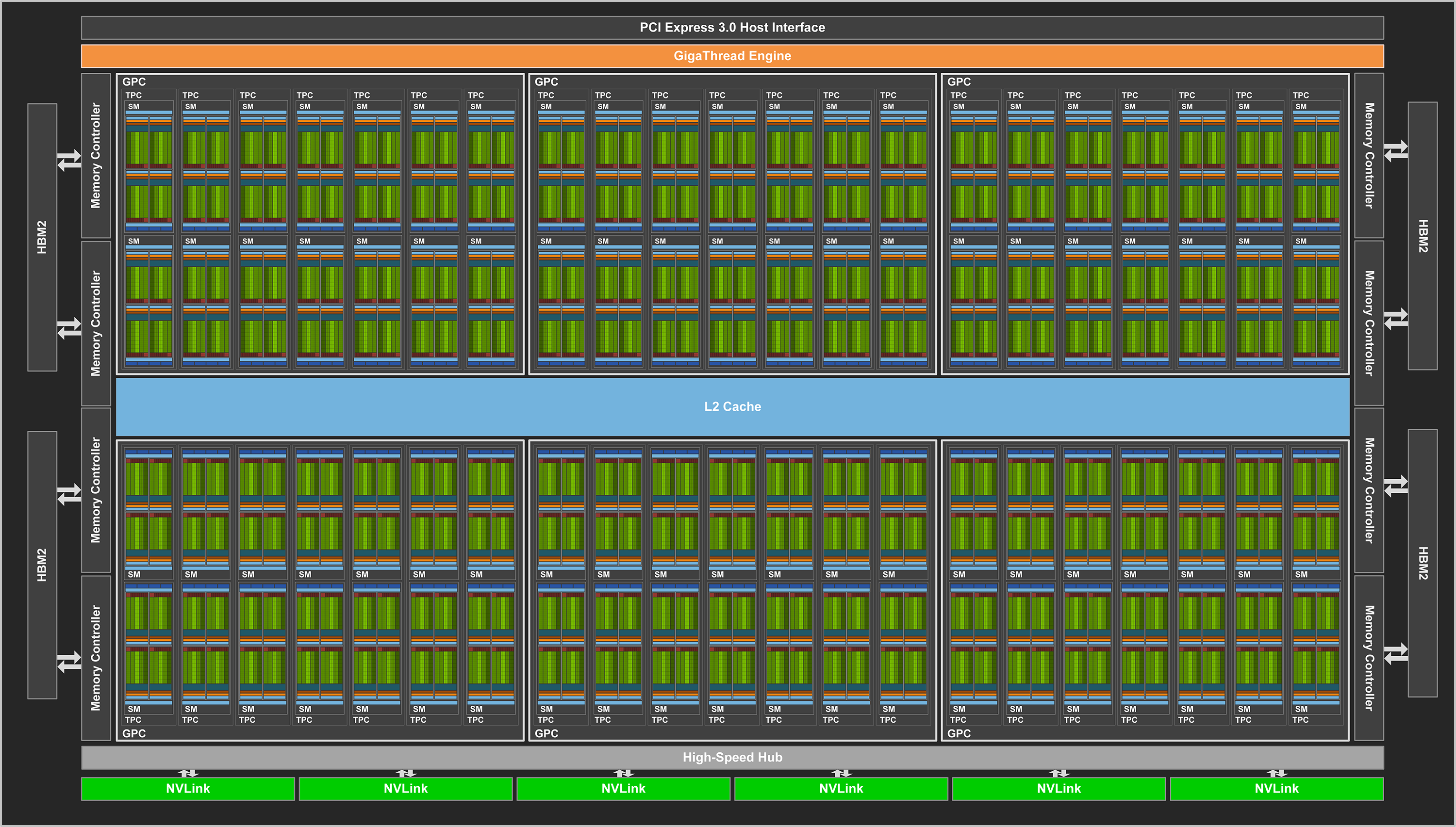
NVIDIA V100 SM
Each SM on the V100 contains 32 FP64 (double-precision) cores, 64 FP32 (single-precision) cores, 64 INT32 cores, and 8 tensor cores. A 128-KB combined memory block for shared memory and L1 cache can be configured to allow up to 96 KB of shared memory. In addition, each SM has 4 texture units which use the (configured size of the) L1 cache.
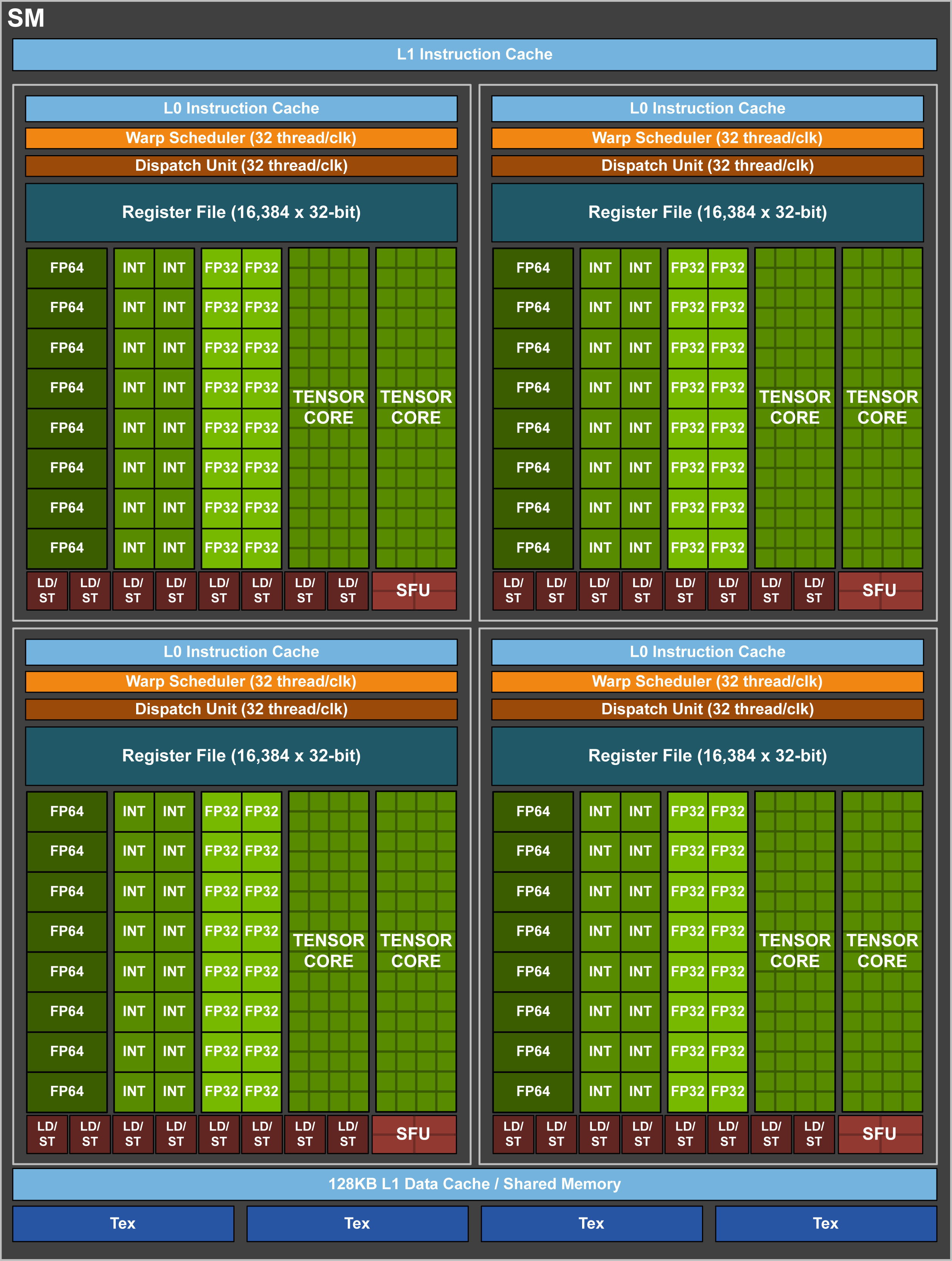
HBM2
Each V100 has access to 16 GB (32GB for high-memory nodes) of high-bandwidth memory (HBM2), which can be accessed at speeds of up to 900 GB/s. Access to this memory is controlled by (8) 512-bit memory controllers, and all accesses to the high-bandwidth memory go through the 6 MB L2 cache.
NVIDIA NVLink
The processors within a node are connected by NVIDIA’s NVLink interconnect. Each link has a peak bandwidth of 25 GB/s (in each direction), and since there are 2 links between processors, data can be transferred from GPU-to-GPU and CPU-to-GPU at a peak rate of 50 GB/s.
Note
The 50-GB/s peak bandwidth stated above is for data transfers in a single direction. However, this bandwidth can be achieved in both directions simultaneously, giving a peak “bi-directional” bandwidth of 100 GB/s between processors.
The figure below shows a schematic of the NVLink connections between the CPU and GPUs on a single socket of a Summit node.
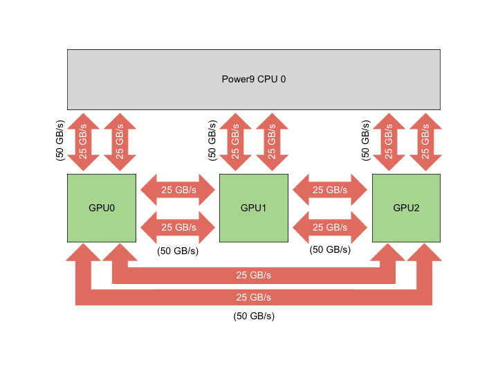
Volta Multi-Process Service
When a CUDA program begins, each MPI rank creates a separate CUDA context on the GPU, but the scheduler on the GPU only allows one CUDA context (and so one MPI rank) at a time to launch on the GPU. This means that multiple MPI ranks can share access to the same GPU, but each rank gets exclusive access while the other ranks wait (time-slicing). This can cause the GPU to become underutilized if a rank (that has exclusive access) does not perform enough work to saturate the resources of the GPU. The following figure depicts such time-sliced access to a pre-Volta GPU.
The Multi-Process Service (MPS) enables multiple processes (e.g. MPI ranks) to concurrently share the resources on a single GPU. This is accomplished by starting an MPS server process, which funnels the work from multiple CUDA contexts (e.g. from multiple MPI ranks) into a single CUDA context. In some cases, this can increase performance due to better utilization of the resources. The figure below illustrates MPS on a pre-Volta GPU.
Volta GPUs improve MPS with new capabilities. For instance, each Volta MPS client (MPI rank) is assigned a “subcontext” that has its own GPU address space, instead of sharing the address space with other clients. This isolation helps protect MPI ranks from out-of-range reads/writes performed by other ranks within CUDA kernels. Because each subcontext manages its own GPU resources, it can submit work directly to the GPU without the need to first pass through the MPS server. In addition, Volta GPUs support up to 48 MPS clients (up from 16 MPS clients on Pascal).

For more information, please see the following document from NVIDIA: https://docs.nvidia.com/deploy/pdf/CUDA_Multi_Process_Service_Overview.pdf
Unified Memory
Unified memory is a single virtual address space that is accessible to any processor in a system (within a node). This means that programmers only need to allocate a single unified-memory pointer (e.g. using cudaMallocManaged) that can be accessed by both the CPU and GPU, instead of requiring separate allocations for each processor. This “managed memory” is automatically migrated to the accessing processor, which eliminates the need for explicit data transfers.
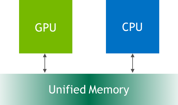
On Pascal-generation GPUs and later, this automatic migration is enhanced with hardware support. A page migration engine enables GPU page faulting, which allows the desired pages to be migrated to the GPU “on demand” instead of the entire “managed” allocation. In addition, 49-bit virtual addressing allows programs using unified memory to access the full system memory size. The combination of GPU page faulting and larger virtual addressing allows programs to oversubscribe the system memory, so very large data sets can be processed. In addition, new CUDA API functions introduced in CUDA8 allow users to fine tune the use of unified memory.
Unified memory is further improved on Volta GPUs through the use of access counters that can be used to automatically tune unified memory by determining where a page is most often accessed.
For more information, please see the following section of NVIDIA’s CUDA Programming Guide: http://docs.nvidia.com/cuda/cuda-c-programming-guide/index.html#um-unified-memory-programming-hd
Independent Thread Scheduling
The V100 supports independent thread scheduling, which allows threads to synchronize and cooperate at sub-warp scales. Pre-Volta GPUs implemented warps (groups of 32 threads which execute instructions in single-instruction, multiple thread - SIMT - mode) with a single call stack and program counter for a warp as a whole.
Within a warp, a mask is used to specify which threads are currently active when divergent branches of code are encountered. The (active) threads within each branch execute their statements serially before threads in the next branch execute theirs. This means that programs on pre-Volta GPUs should avoid sub-warp synchronization; a sync point in the branches could cause a deadlock if all threads in a warp do not reach the synchronization point.
The Tesla V100 introduces warp-level synchronization by implementing warps with a program counter and call stack for each individual thread (i.e. independent thread scheduling).

This implementation allows threads to diverge and synchronize at the sub-warp level using the __syncwarp() function. The independent thread scheduling enables the thread scheduler to stall execution of any thread, allowing other threads in the warp to execute different statements. This means that threads in one branch can stall at a sync point and wait for the threads in the other branch to reach their sync point.
For more information, please see the following section of NVIDIA’s CUDA Programming Guide: http://docs.nvidia.com/cuda/cuda-c-programming-guide/index.html#independent-thread-scheduling-7-x
Tensor Cores
The Tesla V100 contains 640 tensor cores (8 per SM) intended to enable
faster training of large neural networks. Each tensor core performs a
D = AB + C operation on 4x4 matrices. A and B are FP16 matrices,
while C and D can be either FP16 or FP32:
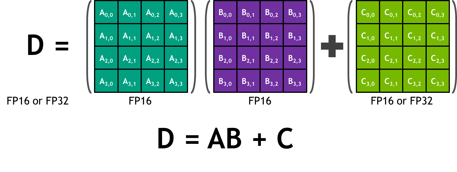
Each of the 16 elements that result from the AB matrix multiplication come from 4 floating-point fused-multiply-add (FMA) operations (basically a dot product between a row of A and a column of B). Each FP16 multiply yields a full-precision product which is accumulated in a FP32 result:
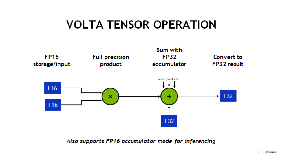
Each tensor core performs 64 of these FMA operations per clock. The 4x4 matrix operations outlined here can be combined to perform matrix operations on larger (and higher dimensional) matrices.
Using the Tensor Cores on Summit
The NVIDIA Tesla V100 GPUs in Summit are capable of over 7TF/s of double-precision and 15 TF/s of single-precision floating point performance. Additionally, the V100 is capable of over 120 TF/s of half-precision floating point performance when using its Tensor Core feature. The Tensor Cores are purpose-built accelerators for half-precision matrix multiplication operations. While they were designed especially to accelerate machine learning workflows, they are exposed through several other APIs that are useful to other HPC applications. This section provides information for using the V100 Tensor Cores.
The V100 Tensor Cores perform a warp-synchronous multiply and accumulate of 16-bit matrices in the form of D = A * B + C. The operands of this matrix multiplication are 16-bit A and B matrices, while the C and D accumulation matrices may be 16 or 32-bit matrices with comparable performance for either precision.
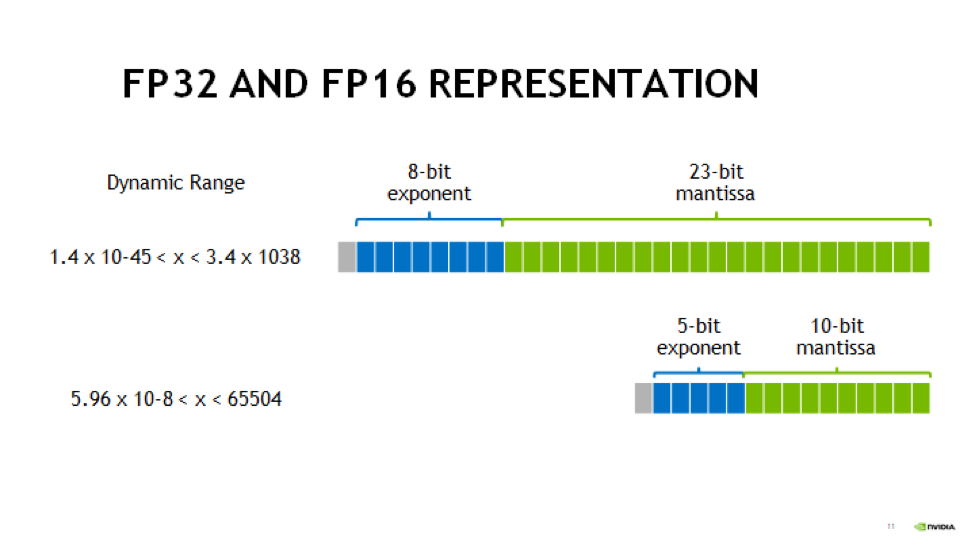
Half precision floating point representation has a dramatically lower range of numbers than Double or Single precision. Half precision representation consists of 1 sign bit, a 5-bit exponent, and a 10-bit mantissa. This results in a dynamic range of 5.96e-8 to 65,504
Tensor Core Programming Models
This section details a variety of high and low-level Tensor Core programming models. Which programming model is appropriate to a given application is highly situational, so this document will present multiple programming models to allow the reader to evaluate each for their merits within the needs of the application.
cuBLAS Library
cuBLAS is NVIDIA’s implementation of the Basic Linear Algebra Subroutines library for GPUs. It contains not only the Level 1, 2, and 3 BLAS routines, but several extensions to these routines that add important capabilities to the library, such as the ability to batch operations and work with varying precisions.
The cuBLAS libraries provides access to the TensorCores using 3 different routines, depending on the application needs. The cublasHgemm routine performs a general matrix multiplication of half-precision matrices. The numerical operands to this routine must be of type half and math mode must be set to CUBLAS_TENSOR_OP_MATH to enable Tensor Core use. Additionally, if the cublasSgemm routine will down-convert from single precision to half precision when the math mode is set to CUBLAS_TENSOR_OP_MATH, enabling simple conversion from SGEMM to HGEMM using Tensor Cores. For either of these two methods the cublasSetMathMode function must be used to change from CUBLAS_DEFAULT_MATH to CUBLAS_TENSOR_OP_MATH mode.
cuBLAS provides a non-standard extension of GEMM with the cublasGemmEx routine, which provides additional flexibility about the data types of the operands. In particular, the A, B, and C matrices can be of arbitrary and different types, with the types of each declared using the Atype, Btype, and Ctype parameters. The algo parameter works similar to the math mode above. If the math mode is set to CUBLAS_TESNOR_OP_MATH and the algo parameter is set to CUBLAS_GEMM_DEFAULT, then the Tensor Cores will be used. If algo is CUBLAS_GEMM_DEFAULT_TENSOR_OP or CUBLAS_GEMM_ALGO{0-15}_TENSOR_OP, then the Tensor Cores will be used regardless of the math setting. The table below outlines the rules stated in the past two paragraphs.
|
|
|
|---|---|---|
|
Disallowed |
Allowed |
|
Allowed |
Allowed |
When using any of these methods to access the Tensor Cores, the M, N, K, LDA, LDB, LDC, and A, B, and C pointers must all be aligned to 8 bytes due to the high bandwidth necessary to utilize the Tensor Cores effective.
Many of the routines listed above are also available in batched form, see the cuBLAS documentation for more information. Advanced users wishing to have increased control over the specifics of data layout, type, and underlying algorithms may wish to use the more advanced cuBLAS-Lt interface. This interface uses the same underlying GPU kernels, but provides developers with a higher degree of control.
Iterative Refinement of Linear Solvers
Iterative Refinement is a technique for performing linear algebra solvers in a reduced precision, then iterating to improve the results and return them to full precision. This technique has been used for several years to use 32-bit math operations and achieve 64-bit results, which often results in a speed-up due to single precision math often have a 2X performance advantage on modern CPUs and many GPUs. NVIDIA and the University of Tennessee have been working to extend this technique to perform operations in half-precision and obtain higher precision results. One such place where this technique has been applied is in calculating an LU factorization of the linear system Ax = B. This operation is dominated by a matrix multiplication operation, which is illustrated in green in the image below. It is possible to perform the GEMM operations at a reduced precision, while leaving the panel and trailing matrices in a higher precision. This technique allows for the majority of the math operations to be done at the higher FP16 throughput. The matrix used in the GEMM is generally not square, which is often the best performing GEMM operation, but is referred to as rank-k and generally still very fast when using matrix multiplication libraries.
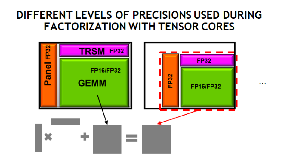
A summary of the algorithm used for calculating in mixed precision is in the following image.

We see in the graph below that it is possible to achieved a 3-4X performance improvement over the double-precision solver, while achieving the same level of accuracy. It has also been observed that the use of Tensor Cores makes the problem more likely to converge than strict half-precision GEMMs due to the ability to accumulate into 32-bit results.

NVIDIA will be shipping official support for IR solvers in their cuSOLVER library in the latter half of 2019. The image below provides estimated release dates, which are subject to change.

Automatic Mixed Precision (AMP) in Machine Learning Frameworks
NVIDIA has a Training With Mixed Precision guide available for developers wishing to explicitly use mixed precision and Tensor Cores in their training of neural networks. This is a good place to start when investigating Tensor Cores for machine learning applications. Developers should specifically read the Optimizing For Tensor Cores section.
NVIDIA has also integrated a technology called Automatic Mixed Precision (AMP) into several common frameworks, TensorFlow, PyTorch, and MXNet at time of writing. In most cases AMP can be enabled via a small code change or via setting and environment variable. AMP does not strictly replace all matrix multiplication operations with half precision, but uses graph optimization techniques to determine whether a given layer is best run in full or half precision.
Examples are provided for using AMP, but the following sections summarize the usage in the three supported frameworks.
TensorFlow
With TensorFlow AMP can be enabled using one of the following techniques.
os.environ['TF_ENABLE_AUTO_MIXED_PRECISION'] = '1'
OR
export TF_ENABLE_AUTO_MIXED_PRECISION=1
Explicit optimizer wrapper available in NVIDIA Container 19.07+, TF 1.14+, TF 2.0:
opt = tf.train.experimental.enable_mixed_precision_graph_rewrite(opt)
PyTorch
Adding the following to a PyTorch model will enable AMP:
model, optimizer = amp.initialize(model, optimizer, opt_level="O1")
with amp.scale_loss(loss, optimizer) as scaled_loss:
  scaled_loss.backward()
MXNet
The code below will enable AMP for MXNet:
amp.init()
amp.init_trainer(trainer)
with amp.scale_loss(loss, trainer) as scaled_loss:
  autograd.backward(scaled_loss)
WMMA
The Warp Matrix Multiply and Accumulate (WMMA) API was introduced in CUDA 9 explicitly for programming the Tesla V100 Tensor Cores. This is a low-level API that supports loading matrix data into fragments within the threads of a warp, applying a Tensor Core multiplication on that data, and then restoring it to the main GPU memory. This API is called within CUDA kernels and all WMMA operations are warp-synchronous, meaning the threads in a warp will leave the operation synchronously. Examples are available for using the WMMA instructions in C++ and CUDA Fortran. The image below demonstrates the general pattern for WMMA usage.
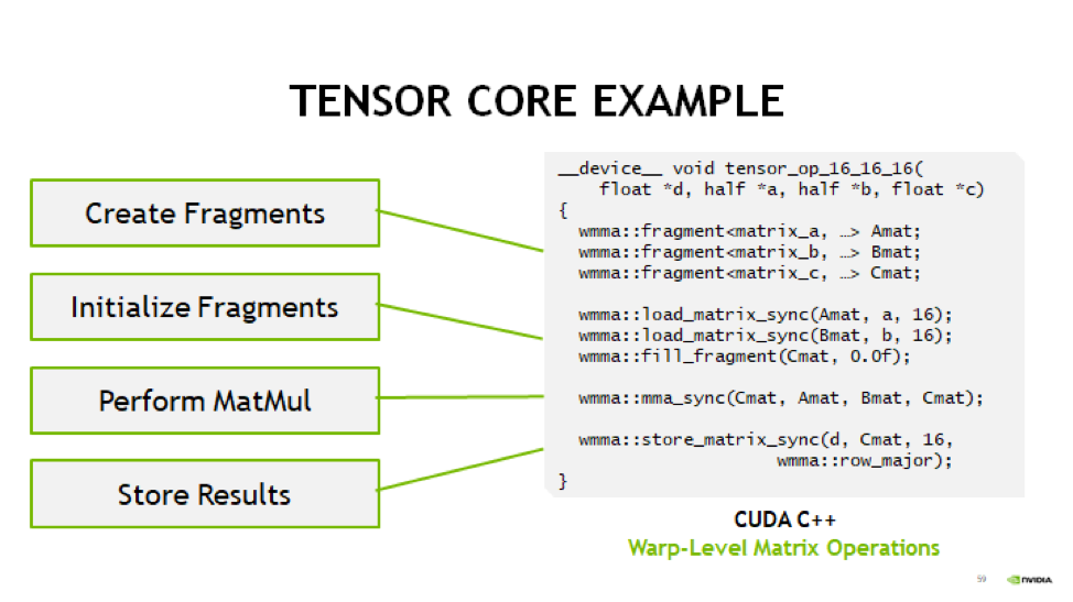
The example above performs a 16-bit accumulate operation, but 32-bit is also supported. Please see the provided samples and the WMMA documentation for more details.
CUDA 10 introduced a lower-level alternative to WMMA with the mma.sync() instruction. This is a very low-level instruction that requires the programmer handle the data movement provided by WMMA explicitly, but is capable of higher performance. Details of mma.sync can be found in the PTX documentation and examples for using this feature via CUTLASS cane be found in the second half of this GTC presentation.
CUTLASS
CUTLASS is an open-source library provided by NVIDIA for building matrix multiplication operations using C++ templates. The goal is to provide performance that is nearly as good as the hand-tuned cuBLAS library, but in a more expressive, composible manner.
The CUTLASS library provides a variety of primitives that are optimized for proper data layout and movement to achieve the maximum possible performance of a matrix multiplation on an NVIDIA GPU. These include iterators for blocking, loading, and storing matrix tiles, plus optimized classes for transforming the data and performing the actual multiplication. CUTLASS provides extensive documentation of these features and examples have been provided. Interested developers are also encouraged to watch the CUTLASS introduction video from GTC2018.
Measuring Tensor Core Utilization
When attempting to use Tensor Cores it is useful to measure and confirm that the Tensor Cores are being used within your code. For implicit use via a library like cuBLAS, the Tensor Cores will only be used above a certain threshold, so Tensor Core use should not be assumed. The NVIDIA Tools provide a performance metric to measure Tensor Core utilization on a scale from 0 (Idle) to 10 (Max) utilization.
When using NVIDIA’s nvprof profiler, one should add the -m tensor_precision_fu_utilization option to measure Tensor Core utilization. Below is the output from measuring this metric on one of the example programs.
$ nvprof -m tensor_precision_fu_utilization ./simpleCUBLAS
==43727== NVPROF is profiling process 43727, command: ./simpleCUBLAS
GPU Device 0: "Tesla V100-SXM2-16GB" with compute capability 7.0

simpleCUBLAS test running..
simpleCUBLAS test passed.
==43727== Profiling application: ./simpleCUBLAS
==43727== Profiling result:
==43727== Metric result:
Invocations                               Metric Name                           Metric Description         Min         Max         Avg
Device "Tesla V100-SXM2-16GB (0)"
    Kernel: volta_h884gemm_128x64_ldg8_nn
          1           tensor_precision_fu_utilization   Tensor-Precision Function Unit Utilization     Low (3)     Low (3)     Low (3)
NVIDIA’s Nsight Compute may also be used to measure tensor core utilization via the sm__pipe_tensor_cycles_active.avg.pct_of_peak_sustained_active metric, as follows:
$ nv-nsight-cu-cli --metrics sm__pipe_tensor_cycles_active.avg.pct_of_peak_sustained_active ./cudaTensorCoreGemm

[  compute_gemm, 2019-Aug-08 12:48:39, Context 1, Stream 7
      Section: Command line profiler metrics
      ----------------------------------------------------------------------
      sm__pipe_tensor_cycles_active.avg.pct_of_peak_sustained_active                    %                       43.44
      ----------------------------------------------------------------------
When to Try Tensor Cores
Tensor Cores provide the potential for an enormous performance boost over full-precision operations, but when their use is appropriate is highly application and even problem independent. Iterative Refinement techniques can suffer from slow or possible a complete lack of convergence if the condition number of the matrix is very large. By using Tensor Cores, which support 32-bit accumulation, rather than strict 16-bit math operations, iterative refinement becomes a viable option in a much larger number of cases, so it should be attempted when an application is already using a supported solver.
Even if iterative techniques are not available for an application, direct use of Tensor Cores may be beneficial if at least the A and B matrices can be constructed from the input data without significant loss of precision. Since the C and D matrices may be 32-bit, the output may have a higher degree of precision than the input. It may be possible to try these operations automatically by setting the math mode in cuBLAS, as detailed above, to determine whether the loss of precision is an acceptable trade-off for increased performance in a given application. If it is, the cublasGemmEx API allows the programmer to control when the conversion to 16-bit occurs, which may result in higher throughput than allowing the cuBLAS library to do the conversion at call time.
Some non-traditional uses of Tensor Cores can come from places where integers that fall within the FP16 range are used in an application. For instance, in “Attacking the Opioid Epidemic: Determining the Epistatic and Pleiotropic Genetic Architectures for Chronic Pain and Opioid Addiction,” a 2018 Gordon Bell Prize-winning paper, the authors used Tensor Cores in place of small integers, allowing them very high performance over performing the same calculation in integer space. This technique is certainly not applicable to all applications, but does show that Tensor Cores may be used in algorithms that might not have been represented by a floating point matrix multiplication otherwise.
Lastly, when performing the training step of a deep learning application it is often beneficial to do at least some of the layer calculations in reduced precision. The AMP technique described above can be tried with little to know code changes, making it highly advisable to attempt in any machine learning application.
Tensor Core Examples and Other Materials
NVIDIA has provided several example codes for using Tensor Cores from a variety of the APIs listed above. These examples can be found on GitHub.
NVIDIA Tensor Core Workshop (August 2018): slides, recording (coming soon)
Tesla V100 Specifications
Compute Capability |
7.0 |
Peak double precision floating point performance |
7.8 TFLOP/s |
Peak single precision floating point performance |
15.7 TFLOP/s |
Single precision CUDA cores |
5120 |
Double precision CUDA cores |
2560 |
Tensor cores |
640 |
Clock frequency |
1530 MHz |
Memory Bandwidth |
900 GB/s |
Memory size (HBM2) |
16 or 32 GB |
L2 cache |
6 MB |
Shared memory size / SM |
Configurable up to 96 KB |
Constant memory |
64 KB |
Register File Size |
256 KB (per SM) |
32-bit Registers |
65536 (per SM) |
Max registers per thread |
255 |
Number of multiprocessors (SMs) |
80 |
Warp size |
32 threads |
Maximum resident warps per SM |
64 |
Maximum resident blocks per SM |
32 |
Maximum resident threads per SM |
2048 |
Maximum threads per block |
1024 |
Maximum block dimensions |
1024, 1024, 64 |
Maximum grid dimensions |
2147483647, 65535, 65535 |
Maximum number of MPS clients |
48 |
Further Reading
For more information on the NVIDIA Volta architecture, please visit the following (outside) links.
Burst Buffer
NVMe (XFS)
Each compute node on Summit has a 1.6TB Non-Volatile Memory (NVMe) storage device (high-memory nodes have a 6.4TB NVMe storage device), colloquially known as a “Burst Buffer” with theoretical performance peak of 2.1 GB/s for writing and 5.5 GB/s for reading. 100GB of each NVMe is reserved for NFS cache to help speed access to common libraries. When calculating maximum usable storage size, this cache and formatting overhead should be considered; We recommend a maximum storage of 1.4TB (6TB for high-memory nodes). The NVMes could be used to reduce the time that applications wait for I/O. Using an SSD drive per compute node, the burst buffer will be used to transfer data to or from the drive before the application reads a file or after it writes a file. The result will be that the application benefits from native SSD performance for a portion of its I/O requests. Users are not required to use the NVMes. Data can also be written directly to the parallel filesystem.
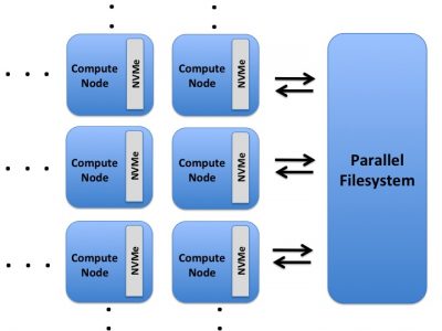
The NVMes on Summit are local to each node.
Current NVMe Usage
Tools for using the burst buffers are still under development. Currently, the user will have access to a writeable directory on each node’s NVMe and then explicitly move data to and from the NVMes with posix commands during a job. This mode of usage only supports writing file-per-process or file-per-node. It does not support automatic “n to 1” file writing, writing from multiple nodes to a single file. After a job completes the NVMes are trimmed, a process that irreversibly deletes data from the devices, so all desired data from the NVMes will need to be copied back to the parallel filesystem before the job ends. This largely manual mode of usage will not be the recommended way to use the burst buffer for most applications because tools are actively being developed to automate and improve the NVMe transfer and data management process. Here are the basic steps for using the BurstBuffers in their current limited mode of usage:
Modify your application to write to /mnt/bb/$USER, a directory that will be created on each NVMe.
Modify either your application or your job submission script to copy the desired data from /mnt/bb/$USER back to the parallel filesystem before the job ends.
Modify your job submission script to include the
-alloc_flags NVMEbsub option. Then on each reserved Burst Buffer node will be available a directory called /mnt/bb/$USER.Submit your bash script or run the application.
Assemble the resulting data as needed.
Interactive Jobs Using the NVMe
The NVMe can be setup for test usage within an interactive job as follows:
bsub -W 30 -nnodes 1 -alloc_flags "NVME" -P project123 -Is bash
The -alloc_flags NVME option will create a directory called /mnt/bb/$USER on
each requested node’s NVMe. The /mnt/bb/$USER directories will be writeable
and readable until the interactive job ends. Outside of a job /mnt/bb/ will
be empty and you will not be able to write to it.
NVMe Usage Example
The following example illustrates how to use the burst buffers (NVMes) by default on Summit. This example uses a submission script, check_nvme.lsf. It is assumed that the files are saved in the user’s GPFS scratch area, /gpfs/alpine/scratch/$USER/projid, and that the user is operating from there as well. Do not forget that for all the commands on NVMe, it is required to use jsrun. This will submit a job to run on one node.
Job submssion script: check_nvme.lsf.
#!/bin/bash
#BSUB -P project123
#BSUB -J name_test
#BSUB -o nvme_test.o%J
#BSUB -W 2
#BSUB -nnodes 1
#BSUB -alloc_flags NVME

#Declare your project in the variable
projid=xxxxx
cd /gpfs/alpine/scratch/$USER/$projid

#Save the hostname of the compute node in a file
jsrun -n 1 echo $HOSTNAME > test_file

#Check what files are saved on the NVMe, always use jsrun to access the NVMe devices
jsrun -n 1 ls -l /mnt/bb/$USER/

#Copy the test_file in your NVMe
jsrun -n 1 cp test_file /mnt/bb/$USER/

#Delete the test_file from your local space
rm test_file

#Check again what the NVMe folder contains
jsrun -n 1 ls -l /mnt/bb/$USER/

#Output of the test_file contents
jsrun -n 1 cat /mnt/bb/$USER/test_file

#Copy the file from the NVMe to your local space
jsrun -n 1 cp /mnt/bb/$USER/test_file .

#Check the file locally
ls -l test_file
To run this example: bsub ./check_nvme.lsf. We could include all the
commands in a script and call this file as a jsrun argument in an interactive
job, in order to avoid changing numbers of processes for all the jsrun
calls. You can see in the table below an example of the differences in a
submission script for executing an application on GPFS and NVMe. In the example,
a binary ./btio reads input from an input file and generates output files.
In this particular case we copy the binary and the input file onto the NVMe, but
this depends on the application as it is not always necessary, we can execute
the binary on the GPFS and write/read the data from NVMe if it is supported by
the application.
Using GPFS |
Using NVMe |
||
|
|
||
|
|
||
|
|
||
|
|
||
|
|
||
|
|
||
|
|
||
|
|
||
|
|||
|
|||
|
|||
|
|||
|
|||
|
|||
When a user occupies more than one compute node, then they are using more NVMes and the I/O can scale linearly. For example in the following plot you can observe the scalability of the IOR benchmark on 2048 compute nodes on Summit where the write performance achieves 4TB/s and the read 11.3 TB/s
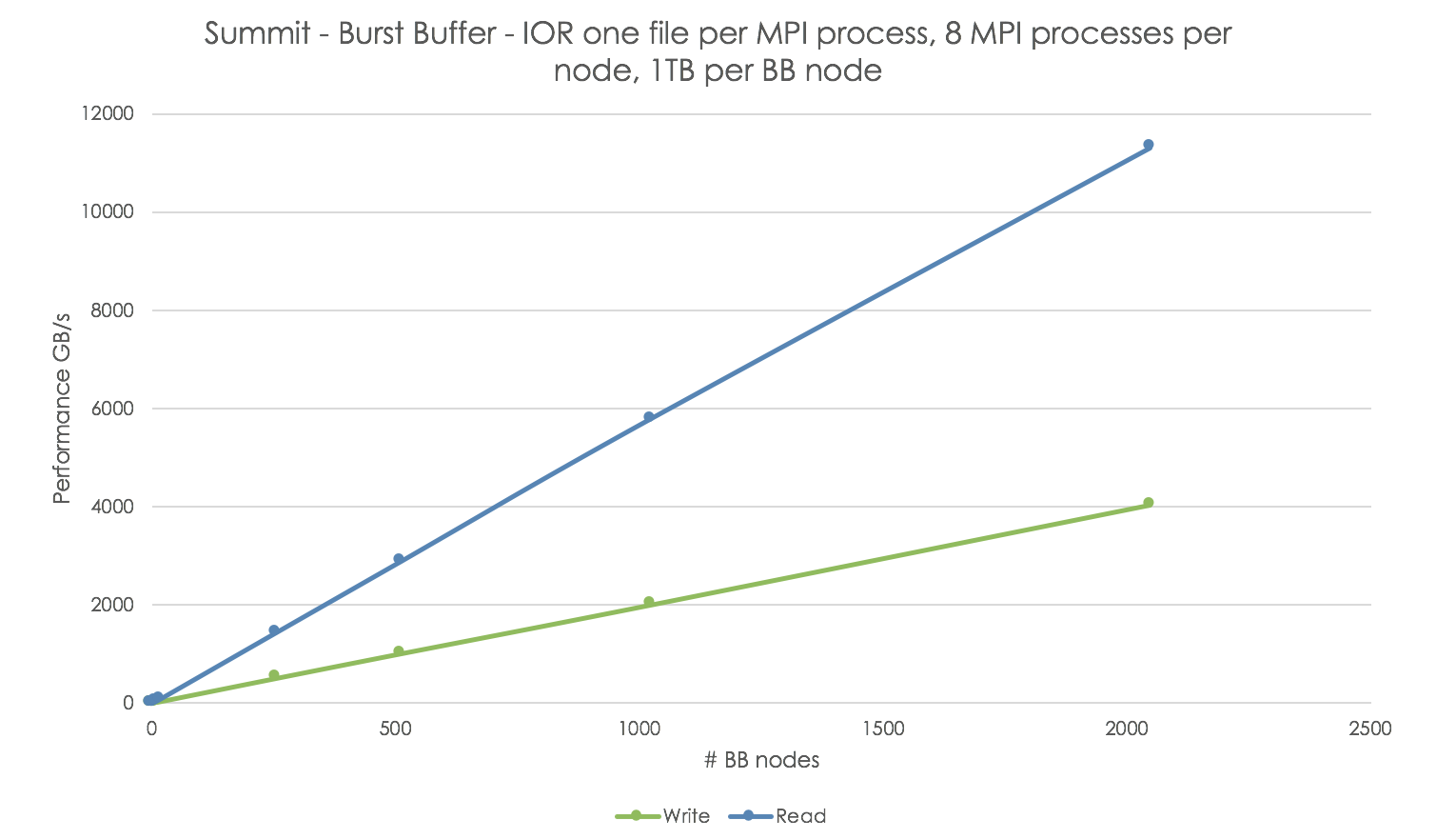
Remember that by default NVMe support one file per MPI process up to one file per compute node. If users desire a single file as output from data staged on the NVMe they will need to construct it. Tools to save automatically checkpoint files from NVMe to GPFS as also methods that allow automatic n to 1 file writing with NVMe staging are under development. Tutorials about NVME: Burst Buffer on Summit (slides, video) Summit Burst Buffer Libraries (slides, video).
Spectral Library
Spectral is a portable and transparent middleware library to enable use of the node-local burst buffers for accelerated application output on Summit. It is used to transfer files from node-local NVMe back to the parallel GPFS file system without the need of the user to interact during the job execution. Spectral runs on the isolated core of each reserved node, so it does not occupy resources and based on some parameters the user could define which folder to be copied to the GPFS. In order to use Spectral, the user has to do the following steps in the submission script:
Request Spectral resources instead of NVMe
Declare the path where the files will be saved in the node-local NVMe (PERSIST_DIR)
Declare the path on GPFS where the files will be copied (PFS_DIR)
Execute the script spectral_wait.py when the application is finished in order to copy the files from NVMe to GPFS
The following table shows the differences of executing an application on GPFS, NVMe, and NVMe with Spectral. This example is using one compute node. We copy the executable and input file for the NVMe cases but this is not always necessary. Depending on the application, you could execute the binary from the GPFS and save the output files on NVMe. Adjust your parameters to copy, if necessary, the executable and input files onto all the NVMe devices.
Using GPFS |
Using NVMe |
Using NVME with Spectral library |
|
|
|
|
|
|
|
|
|
|
|
|
|
|
|
|
|
|
|
|
|
|
|
|
|
||
|
|
|
|
||
|
||
|
|
|
|
|
|
|
|
|
|
|
|
|
|
When the Spectral library is not used, any output data produced has to be copied back from NVMe. You can observe that with the Spectral library there is no reason to explicitly ask for the data to be copied to GPFS as it is done automatically through the spectral_wait.py script. Also a log file called spectral.log will be created with information on the files that were copied.
Known Issues
Last Updated: 07 February 2023
Open Issues
HIP code cannot be built using CMake using hip::host/device or HIP language support
Using the hip-cuda/5.1.0 module on Summit, applications cannot build using a CMakeLists.txt that requires HIP language support or references the hip::host and hip::device identifiers. There is no known workaround for this issue. Applications wishing to compile HIP code with CMake need to avoid using HIP language support or hip::host and hip::device identifiers.
Unsupported CUDA versions do not work with GPU-aware MPI
Although there are newer CUDA modules on Summit, cuda/11.0.3 is the latest version that is officially supported by the version of IBM’s software stack installed on Summit. When loading the newer CUDA modules, a message is printed to the screen stating that the module is for “testing purposes only”. These newer unsupported CUDA versions might work with some users’ applications, but importantly, they are known not to work with GPU-aware MPI.
HIP does not currently work with GPU-aware MPI
Using the hip-cuda/5.1.0 module on Summit requires CUDA v11.4.0 or later. However, only CUDA v11.0.3 and earlier currently support GPU-aware MPI, so GPU-aware MPI is currently not available when using HIP on Summit.
MPS does not currently work with codes compiled with post 11.0.3 CUDA
Any codes compiled with post 11.0.3 CUDA (cuda/11.0.3) will not work with MPS enabled (-alloc_flags "gpumps") on Summit. The code will hang indefinitely. CUDA v11.0.3 is the latest version that is officially supported by IBM’s software stack installed on Summit. We are continuing to look into this issue.
System not sourcing .bashrc, .profile, etc. files as expected
Some users have noticed that their login shells, batch jobs, etc. are not sourcing shell run control files as expected. This is related to the way bash is initialized. The initialization process is discussed in the INVOCATION section of the bash manpage, but is summarized here.
Bash sources different files based on two attributes of the shell: whether or not it’s a login shell, and whether or not it’s an interactive shell. These attributes are not mutually exclusive (so a shell can be “interactive login”, “interactive non-login”, etc.):
If a shell is an interactive login shell (i.e. an ssh to the system) or a non-interactive shell started with the
--loginoption (say, a batch script with#!/bin/bash --loginas the first line), it will source/etc/profileand will then search your home directory for~/.bash_profile,~/.bash_login, and~/.profile. It will source the first of those that it finds (once it sources one, it stops looking for the others).If a shell is an interactive, non-login shell (say, if you run ‘bash’ in your login session to start a subshell), it will source
~/.bashrcIf a shell is a non-interactive, non-login shell, it will source whatever file is defined by the
$BASH_ENVvariable in the shell from which it was invoked.
In any case, if the files listed above that should be sourced in a particular situation do not exist, it is not an error.
On Summit and Andes, batch-interactive jobs using bash (i.e. those submitted with bsub -Is or salloc) run as interactive, non-login shells (and therefore source ~/.bashrc, if it exists). Regular batch jobs using bash on those systems are non-interactive, non-login shells and source the file defined by the variable $BASH_ENV in the shell from which you submitted the job. This variable is not set by default, so this means that none of these files will be sourced for a regular batch job unless you explicitly set that variable.
Some systems are configured to have additional files in /etc sourced, and sometimes the files in /etc look for and source files in your home directory such as ~/.bashrc, so the behavior on any given system may seem to deviate a bit from the information above (which is from the bash manpage). This can explain why jobs (or other shells) on other systems you’ve used have sourced your .bashrc file on login.
Improper permissions on ~/.ssh/config cause job state flip-flop/jobs ending in suspended state
Improper permissions on your SSH configuration file (~/.ssh/config) will cause jobs to alternate between pending & running states until the job ultimately ends up in a PSUSP state.
LSF uses SSH to communicate with nodes allocated to your job, and in this case the improper permissions (i.e. write permission for anyone other than the user) cause SSH to fail, which in turn causes the job launch to fail. Note that SSH only checks the permissions of the configuration file itself. Thus, even if the ~/.ssh/ directory itself grants no group or other permissions, SSH will fail due to permissions on the configuration file.
To fix this, use a more secure permission setting on the configuration file. An appropriate setting would be read and write permission for the user and no other permissions. You can set this with the command chmod 600 ~/.ssh/config.
Setting TMPDIR causes JSM (jsrun) errors / job state flip-flop
Setting the TMPDIR environment variable causes jobs to fail with JSM
(jsrun) errors and can also cause jobs to bounce back and forth between
eligible and running states until a retry limit has been reached and the job is
placed in a blocked state (NOTE: This “bouncing” of job state can be caused for
multiple reasons. Please see the known issue Jobs suspended due to retry limit
/ Queued job flip-flops between queued/running states if you are not setting
TMPDIR). A bug has been filed with IBM to address this issue.
When TMPDIR is set within a running job (i.e., in an interactive session or
within a batch script), any attempt to call jsrun will lead to a job
failure with the following error message:
Error: Remote JSM server is not responding on host batch503-25-2020 15:29:45:920 90012 main: Error initializing RM connection. Exiting.
When TMPDIR is set before submitting a job (i.e., in the shell/environment
where a job is submitted from), the job will bounce back and forth between a
running and eligible state until its retry limit has been reached and the job
will end up in a blocked state. This is true for both interactive jobs and jobs
submitted with a batch script, but interactive jobs will hang without dropping
you into your interactive shell. In both cases, JSM log files (e.g.,
jsm-lsf-wait.username.1004985.log) will be created in the location set for
TMPDIR containing the same error message as shown above.
Segfault when running executables on login nodes
Executing a parallel binary on the login node or a batch node without using the
job step launcher jsrun will result in a segfault.
This also can be encountered when importing parallel Python libraries like
mpi4py and h5py directly on these nodes.
The issue has been reported to IBM. The current workaround is to run the binary
inside an interactive or batch job via jsrun.
Nsight Compute cannot be used with MPI programs
When profiling an MPI application using NVIDIA Nsight Compute, like the following, you may see an error message in Spectrum MPI that aborts the program:
jsrun -n 1 -a 1 -g 1 nv-nsight-cu-cli ./a.out

Error: common_pami.c:1049 - ompi_common_pami_init() Unable to create PAMI client (rc=1)
--------------------------------------------------------------------------
No components were able to be opened in the pml framework.

This typically means that either no components of this type were
installed, or none of the installed components can be loaded.
Sometimes this means that shared libraries required by these
components are unable to be found/loaded.

Host:      <host>
Framework: pml
--------------------------------------------------------------------------
PML pami cannot be selected
This is due to an incompatibility in the 2019.x versions of Nsight Compute with Spectrum MPI. As a workaround, you can disable CUDA hooks in Spectrum MPI using
jsrun -n 1 -a 1 -g 1 --smpiargs="-disable_gpu_hooks" nv-nsight-cu-cli ./a.out
Unfortunately, this is incompatible with using CUDA-aware MPI in your application.
This will be resolved in a future release of CUDA.
CUDA hook error when program uses CUDA without first calling MPI_Init()
Serial applications, that are not MPI enabled, often face the following issue when compiled with Spectrum MPI’s wrappers and run with jsrun:
CUDA Hook Library: Failed to find symbol mem_find_dreg_entries, ./a.out: undefined symbol: __PAMI_Invalidate_region
The same issue can occur if CUDA API calls that interact with the GPU (e.g. allocating memory) are called before MPI_Init() in an MPI enabled application. Depending on context, this error can either be harmless or it can be fatal.
The reason this occurs is that the PAMI messaging backend, used by Spectrum MPI by default, has a “CUDA hook” that records GPU memory allocations. This record is used later during CUDA-aware MPI calls to efficiently detect whether a given message is sent from the CPU or the GPU. This is done by design in the IBM implementation and is unlikely to be changed.
There are two main ways to work around this problem. If CUDA-aware MPI is not a relevant factor for your work (which is naturally true for serial applications) then you can simply disable the CUDA hook with:
--smpiargs="-disable_gpu_hooks"
as an argument to jsrun. Note that this is not compatible with the -gpu
argument to --smpiargs, since that is what enables CUDA-aware MPI and
the CUDA-aware MPI functionality depends on the CUDA hook.
If you do need CUDA-aware MPI functionality, then the only known working solution to this problem is to refactor your code so that no CUDA calls occur before MPI_Init(). (This includes any libraries or programming models such as OpenACC or OpenMP that would use CUDA behind the scenes.) While it is not explicitly codified in the standard, it is worth noting that the major MPI implementations all recommend doing as little as possible before MPI_Init(), and this recommendation is consistent with that.
Spindle is not currently supported
Users should not use USE_SPINDLE=1 or LOAD_SPINDLE=1 in their
~/.jsm.conf file at this time. A bug has been filed with IBM to
address this issue.
Spectrum MPI tunings needed for maximum bandwidth
By default, Spectrum MPI is configured for minimum latency. If your application needs maximum bandwidth, the following settings are recommended:
$ export PAMI_ENABLE_STRIPING=1
$ export PAMI_IBV_ADAPTER_AFFINITY=1
$ export PAMI_IBV_DEVICE_NAME="mlx5_0:1,mlx5_3:1"
$ export PAMI_IBV_DEVICE_NAME_1="mlx5_3:1,mlx5_0:1"
Debugging slow application startup or slow performance
In order for debugging and profiling tools to work, you need to unload Darshan
$ module unload darshan-runtime
Spectrum MPI provides a tracing library that can be helpful to gather
more detail information about the MPI communication of your job. To
gather MPI tracing data, you can set
export OMPI_LD_PRELOAD_POSTPEND=$OLCF_SPECTRUM_MPI_ROOT/lib/libmpitrace.so
in your environment. This will generate profile files with timings for
the individual processes of your job.
In addition, to debug slow startup JSM provides the option to create a
progress file. The file will show information that can be helpful to
pinpoint if a specific node is hanging or slowing down the job step
launch. To enable it, you can use: jsrun --progress
./my_progress_file_output.txt.
-a flag ignored when using a jsrun resource set file with -U
When using file-based specification of resource sets with jsrun -U,
the -a flag (number of tasks per resource set) is ignored. This has
been reported to IBM and they are investigating. It is generally
recommended to use jsrun explicit resource files (ERF) with
--erf_input and --erf_output instead of -U.
Jobs suspended due to retry limit / Queued job flip-flops between queued/running states
Some users have reported seeing their jobs transition from the normal
queued state, into a running state, and then back again to queued.
Sometimes this can happen multiple times. Eventually, internal limits in
the LSF scheduler will be reached, at which point the job will no longer
be eligible for running. The bhist command can be used to see if a job
is cycling between running and eligible states. The pending reason given
by bhist can also be useful to debug. This can happen due to
modifications that the user has made to their environment on the system,
incorrect SSH key setup, attempting to load unavailable/broken modules.
or system problems with individual nodes. When jobs are observed to
flip-flop between running and queued, and/or become ineligible without
explanation, then deeper investigation is required and the user should
write to help@olcf.ornl.gov.
jsrun explicit resource file (ERF) output format error
jsrun’s option to create an explicit resource file (--erf_output) will
incorrectly create a file with one line per rank. When reading the file
in with (--erf_input) you will see warnings for overlapping resource
sets. This issue has been reported. The workaround is to manually
update the created ERF file to contain a single line per resource set
with multiple ranks per line.
jsrun latency priority capitalization allocates incorrect resources
jsrun’s latency priority (-l) flag can be given lowercase values
(i.e. gpu-cpu) or capitalized values (i.e. GPU-CPU).
Expected behavior:
When capitalized, jsrun should not compromise on the resource layout, and will wait to begin the job step until the ideal resources are available. When given a lowercase value, jsrun will not wait, but initiate the job step with the most ideal layout as is available at the time. This also means that when there’s no resource contention, such as running a single job step at a time, capitalization should not matter, as they should both yield the same resources.
Actual behavior:
Capitalizing the latency priority value may allocate incorrect resources, or even cause the job step to fail entirely.
Recommendation:
It is currently recommended to only use the lowercase values to (
-l/--latency_priority). The system default is: gpu-cpu,cpu-mem,cpu-cpu. Since this ordering is used implicitly when the-lflag is omitted, this issue only impacts submissions which explicitly include a latency priority in the jsrun command.
Error when using complex datatypes with MPI Collectives and GPUDirect
Users have reported errors when using complex datatypes with MPI Collectives and GPUDirect:
jsrun --smpiargs="-gpu" -n 6 -a 1 -g 1   ./a.out
[h35n05:113506] coll:ibm:allreduce: GPU awareness in PAMI requested. It is not safe to defer to another component.
[h35n05:113506] *** An error occurred in MPI_Allreduce
[h35n05:113506] *** reported by process [3199551009,2]
[h35n05:113506] *** on communicator MPI_COMM_WORLD
[h35n05:113506] *** MPI_ERR_UNSUPPORTED_OPERATION: operation not supported
[h35n05:113506] *** MPI_ERRORS_ARE_FATAL (processes in this communicator will now abort,
[h35n05:113506] ***    and potentially your MPI job)
[h35n05:113509] coll:ibm:allreduce: GPU awareness in PAMI requested. It is not safe to defer to another component.
This is a known issue with libcoll and the SMPI team is working to
resolve it. In the meantime, a workaround is to treat the complex array
as a real array with double the length if the operation is not
MPI_Prod. Note: This requires code modification. An alternative
workaround is to disable IBM optimized collectives. This will impact
performance however but requires no code changes and should be correct
for all MPI_Allreduce operations. You can do this by adding the
following option to your jsrun command line:
--smpiargs="-HCOLL -FCA -mca coll_hcoll_enable 1 -mca coll_hcoll_np 0
-mca coll ^basic -mca coll ^ibm -async"
Error when using ERF
Explicit Resource Files provide even more fine-granied control over how processes are mapped onto compute nodes. Users have reported errors when using ERF on Summit:
Failed to bind process to ERF smt array, err: Invalid argument
This is a known issue with the current version of jsrun.
Resolved Issues
‘Received msg header indicates a size that is too large’ error message from Spectrum MPI
If you get an error message that looks like:
A received msg header indicates a size that is too large:
 Requested size: 25836785
 Size limit: 16777216
If you believe this msg is legitimate, please increase the
max msg size via the ptl_base_max_msg_size parameter.
This can be resolved by setting export PMIX_MCA_ptl_base_max_msg_size=18 where the value is size in MB. Setting it to 18 or higher usually works. The default if its not explicitly set is around 16 MB.
JSM Fault Tolerance causes jobs to fail to start
Adding FAULT_TOLERANCE=1 in your individual ~/.jsm.conf file,
will result in LSF jobs failing to successfully start.
The following issues were resolved with the July 16, 2019 software upgrade:
Default nvprof setting clobbers LD_PRELOAD, interfering with SpectrumMPI (Resolved: July 16, 2019)
CUDA 10 adds a new feature to profile CPU side OpenMP constructs (see
https://docs.nvidia.com/cuda/profiler-users-guide/index.html#openmp).
This feature is enabled by default and has a bug which will cause it to
overwrite the contents of LD_PRELOAD. SpectrumMPI requires a library
(libpami_cuda_hook.so) to be preloaded in order to function. All MPI
applications on Summit will break when run in nvprof with default
settings. The workaround is to disable the new OpenMP profiling feature:
$ jsrun nvprof --openmp-profiling off
CSM-based launch is not currently supported (Resolved: July 16, 2019)
Users should not use JSMD_LAUNCH_MODE=csm in their ~/.jsm.conf
file at this time. A bug has been filed with IBM to address this issue.
Parallel I/O crash on GPFS with latest MPI ROMIO
In some cases with large number of MPI processes when there is not enough memory available on the compute node, the Abstract-Device Interface for I/O (ADIO) driver can break with this error:
Out of memory in file ../../../../../../../opensrc/ompi/ompi/mca/io/romio321/romio/adio/ad_gpfs/ad_gpfs_rdcoll.c, line 1178
The solution is to declare in your submission script:
export GPFSMPIO_COMM=1
This command will use non-blocking MPI calls and not MPI_Alltoallv for exchange of data between the MPI I/O aggregators which requires significant more amount of memory.
The following issues were resolved with the May 21, 2019 upgrade:
-g flag causes internal compiler error with XL compiler (Resolved: May 21, 2019)
Some users have reported an internal compiler error when compiling their code with XL with the `-g` flag. This has been reported to IBM and they are investigating.
Note
This bug was fixed in xl/16.1.1-3
Issue with CUDA Aware MPI with >1 resource set per node (Resolved: May 21, 2019)
Attempting to run an application with CUDA-aware MPI using more than one resource set per node with produce the following error on each MPI rank:
/__SMPI_build_dir__________________________________________/ibmsrc/pami/ibm-pami/buildtools/pami_build_port/../pami/components/devices/ibvdevice/CudaIPCPool.h:300:
[0]Error opening IPC Memhandle from peer:1, invalid argument
CUDA level IPC failure: this has been observed in environments where cgroups separate the visible GPUs between ranks. The option -x PAMI_DISABLE_IPC=1 can be used to disable CUDA level IPC.[:] *** Process received signal ***
Spectrum MPI relies on CUDA Inter-process Communication (CUDA IPC) to provide fast on-node between GPUs. At present this capability cannot function with more than one resource set per node.
Set the environment variable
PAMI_DISABLE_IPC=1to force Spectrum MPI to not use fast GPU Peer-to-peer communication. This option will allow your code to run with more than one resource set per host, but you may see slower GPU to GPU communication.Run in a single resource set per host, i.e. with
jsrun --gpu_per_rs 6
If on-node MPI communication between GPUs is critical to your
application performance, option B is recommended but you’ll need to set
the GPU affinity manually. This could be done with an API call in your
code (e.g. cudaSetDevice), or by using a wrapper script.
Simultaneous backgrounded jsruns (Resolved: May 21, 2019)
We have seen occasional errors from batch jobs with multiple simultaneous backgrounded jsrun commands. Jobs may see pmix errors during the noted failures.
The following issue was resolved with the software default changes from March 12, 2019 that set Spectrum MPI 10.2.0.11 (20190201) as default and moved ROMIO to version 3.2.1:
Slow performance using parallel HDF5 (Resolved: March 12, 2019)
A performance issue has been identified using parallel HDF5 with the
default version of ROMIO provided in
spectrum-mpi/10.2.0.10-20181214. To fully take advantage of parallel
HDF5, users need to switch to the newer version of ROMIO and use ROMIO
hints. The following shows recommended variables and hints for a 2 node
job. Please note that hints must be tuned for a specific job.
$ module unload darshan-runtime
$ export OMPI_MCA_io=romio321
$ export ROMIO_HINTS=./my_romio_hints
$ cat $ROMIO_HINTS
romio_cb_write enable
romio_ds_write enable
cb_buffer_size 16777216
cb_nodes 2
Job hangs in MPI_Finalize (Resolved: March 12, 2019)
There is a known issue in Spectrum MPI 10.2.0.10 provided by the
spectrum-mpi/10.2.0.10-20181214 modulefile that causes a hang in
MPI_Finalize when ROMIO 3.2.1 is being used and the
darshan-runtime modulefile is loaded. The recommended and default
Spectrum MPI version as of March 3, 2019 is Spectrum MPI 10.2.0.11
provided by the spectrum-mpi/10.2.0.11-20190201 modulefile. If you
are seeing this issue, please make sure that you are using the latest
version of Spectrum MPI. If you need to use a previous version of
Spectrum MPI, your options are:
Unload the
darshan-runtimemodulefile.Alternatively, set
export OMPI_MCA_io=romio314in your environment to use the previous version of ROMIO. Please note that this version has known performance issues with parallel HDF5 (see “Slow performance using parallel HDF5” issue below).
The following issues were resolved with the February 19, 2019 upgrade:
Job step cgroups are not currently supported (Resolved: February 19, 2019)
A regression was introduced in JSM 10.02.00.10rtm2 that prevents job
step cgroups from being created as a result, JSM, is defaulting to
setting CUDA_VISIBLE_DEVICES in order to allocate GPUs to specific
resource sets. Because of this issue, even if using --gpu_per_rs 0
or -g 0, every resource set in the step will be able to see all 6
GPUs in a node.
JSM stdio options do not create files (Resolved: February 19, 2019)
When using --stdio_stdout or --stdio_stderr users must use
absolute paths. Using relative paths (e.g. ./my_stdout) will not
successfully create the file in the user’s current working directory. An
bug has been filed with IBM to fix this issue and allow relative paths.
JSM crash when using different number of resource sets per host (Resolved: February 19, 2019)
In some cases users will encounter a segmentation fault when running job steps that have uneven number of resource sets per node. For example:
$ jsrun --nrs 41 -c 21 -a 1 --bind rs ./a.out
[a03n07:74208] *** Process received signal ***
[a03n07:74208] Signal: Segmentation fault (11)
[a03n07:74208] Signal code: Address not mapped (1)
[a03n07:74208] Failing at address: (nil)
...
As a workaround, two environment variables are set as default in the
user environment PAMI_PMIX_USE_OLD_MAPCACHE=1 and
OMPI_MCA_coll_ibm_xml_disable_cache=1.
CUDA 10.1 Known Issues
Intermittent failures with `nvprof` (Identified: July 11, 2019)
We are seeing an intermittent issue that causes an error when profiling a code using nvprof from CUDA 10.1.168. We have filed a bug with NVIDIA (NV bug 2645669) and they have reproduced the problem. An update will be posted when a fix becomes available.
When this issue is encountered, the profiler will exit with the following error message:
==99756== NVPROF is profiling process 99756, command: ./a.out
==99756== Error: Internal profiling error 4306:999.
======== Profiling result:
======== Metric result:
MPI annotation may cause segfaults with applications using MPI_Init_thread
Users on Summit can have MPI calls automatically annotated in nvprof
timelines using the nvprof --annotate-mpi openmpi option. If the
user calls MPI_Init_thread instead of MPI_Init, nvprof may
segfault, as MPI_Init_thread is currently not being wrapped by
nvprof. The current alternative is to build and follow the
instructions from
https://github.com/NVIDIA/cuda-profiler/tree/mpi_init_thread.
cudaMemAdvise before context creation leads to a kernel panic
There is a (very rare) driver bug involving cudaManagedMemory that can
cause a kernel panic. If you encounter this bug, please contact the
OLCF User Support team. The easiest
mitigation is for the user code to initialize a context on every GPU
with which it intends to interact (for example by calling
cudaFree(0) while each device is active).
Some uses of Thrust complex vectors fail at compile time with warnings of identifiers being undefined in device code
This issue comes from the fact that std::complex is not
__host__/__device__ annotated, so all its functions are
implicitly __host__. There is a mostly simple workaround, assuming
this is compiled as C++11: in complex.h and complex.inl,
annotate the functions that deal with std::complex as
__host__ __device__ (they are the ones that are annotated only as
__host__ right now), and then compile with
--expt-relaxed-constexpr.
Users that encounter this issue, can use
the following workaround. copy the entirety of
${OLCF_CUDA_ROOT}/include/thrust to a private location, make the
above edits to thrust/complex.h and
thrust/detail/complex/complex.inl, and then add that to your include
path:
$ nvcc -ccbin=g++ --expt-relaxed-constexpr assignment.cu -I./
A permanent fix of this issue is expected in the version of Thrust packed with CUDA 10.1 update 1
Breakpoints in CUDA kernels recommendation
cuda-gdb allows for breakpoints to be set inside CUDA kernels to
inspect the program state on the GPU. This can be a valuable debugging
tool but breaking inside kernels does incur significant overhead that
should be included in your expected runtime.
The time required to hit a breakpoint inside a CUDA kernel depends on how many CUDA threads are used to execute the kernel. It may take several seconds to stop at kernel breakpoints for very large numbers of threads. For this reason, it is recommended to choose breakpoints judiciously, especially when running the debugger in “batch” or “offline” mode where this overhead may be misperceived as the code hanging. If possible, debugging a smaller problem size with fewer active threads can be more pleasant.
Scalable Protected Infrastructure (SPI)
The OLCF’s Scalable Protected Infrastructure (SPI) provides resources and protocols that enable researchers to process protected data at scale. The SPI is built around a framework of security protocols that allows researchers to process large datasets containing private information. Using this framework researchers can use the center’s large HPC resources to compute data containing protected health information (PHI), personally identifiable information (PII), data protected under International Traffic in Arms Regulations, and other types of data that require privacy.
The SPI utilizes a mixture of existing resources combined with specialized resources targeted at SPI workloads. Because of this, many processes used within the SPI are very similar to those used for standard non-SPI. This page lists the differences you may see when using OLCF resources to execute SPI resources.
The SPI provides access to the OLCF’s Summit resource for compute. To safely separate SPI and non-SPI workflows, SPI workflows must use a separate login node named Citadel. Because Citadel is largely a front end for Summit, you can use the Summit documentation when using Citadel. The SPI page can be used to see notable differences when using the Citadel resource.
Training System (Ascent)
Note
Ascent is a training system that is not intended to be used as an OLCF user resource. Access to the system is only obtained through OLCF training events.
Ascent is an 18-node stand-alone system with the same architecture as Summit (see Summit Nodes section above), so most of this Summit User Guide can be referenced for Ascent as well. However, aside from the number of compute nodes, there are other differences between the two systems. Most notably, Ascent sits in the NCCS Open Security Enclave, which is subject to fewer restrictions than the Moderate Security Enclave that systems such as Summit belong to. This means that participants in OLCF training events can go through a streamlined version of the approval process before gaining access to the system. The remainder of this section of the user guide describes “Ascent-specific” information intended for participants of OLCF training events.
File Systems
It is important to note that because Ascent sits in the NCCS Open Security Enclave, it also mounts different file systems than Summit. These file systems provide both user-affiliated and project-affiliated storage areas for each user.
NFS Directories
Upon logging into Ascent, users will be placed in their own personal
home (NFS) directory, /ccsopen/home/[userid], which can only be
accessed by that user. Users also have access to an NFS project
directory, /ccsopen/proj/[projid], which is visible to all members
of a project. Both of these NFS directories are commonly used to store
source code and build applications.
GPFS Directories
Users also have access to a (GPFS) parallel file system, called wolf,
which is where data should be written when running on Ascent’s compute
nodes. Under /gpfs/wolf/[projid], there are 3 directories:
$ ls /gpfs/wolf/[projid]
proj-shared  scratch  world-shared
proj-sharedcan be accessed by all members of a project.scratchcontains directories for each user of a project and only that user can access their own directory.world-sharedcan be accessed by any users on the system in any project.
Obtaining Access to Ascent
Note
Ascent is a training system that is not intended to be used as an OLCF user resource. Access to the system is only obtained through OLCF training events.
This sub-section describes the process of obtaining access to Ascent for an OLCF training event. Please follow the steps below to request access.
Step 1: Go to the myOLCF Account Application Form
Once on the form, linked above, fill in the project ID in the “Enter the Project ID of the project you wish to join” field and click “Next”.
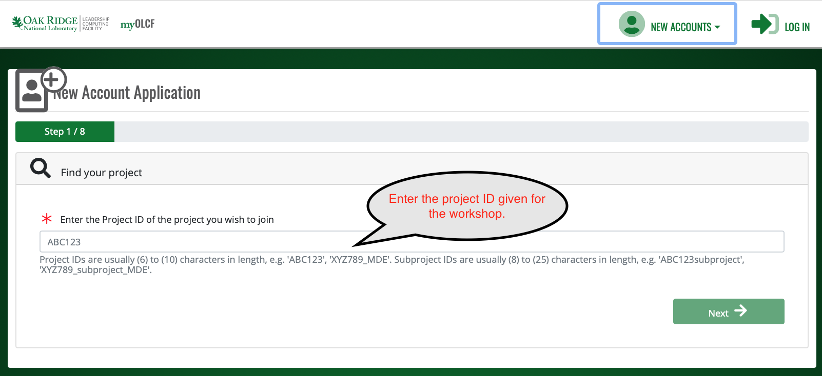
After you enter the Project ID, use the sliders to select “Yes” for OLCF as the Project Organization and select “Yes” for Open as the Security Enclave.
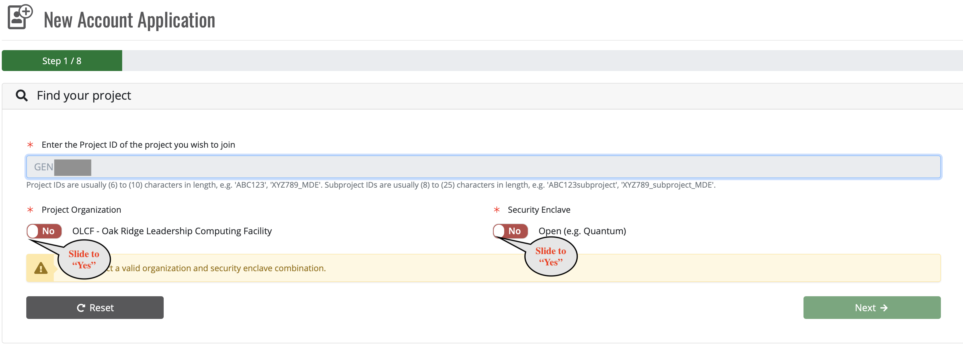
The next screen will show you some information about the project, you don’t need to change anything, just click “Next”.
Fill in your personal information and then click “Next”.
Fill in your shipping information and then click “Next”.
Fill in your Employment/Institution Information. If you are student please use your school affiliation for both “Employer” and “Funding Source”. If you are a student and you do not see your school listed, choose “other” for both “Employer” and “Funding Source” and then manually enter your school affiliation in the adjacent fields. Click “Next” when you are done.
On the Project information screen fill the “Proposed Contribution to Project” with “Participating in OLCF training.” Leave all the questions about the project set to “no” and click “Next”.
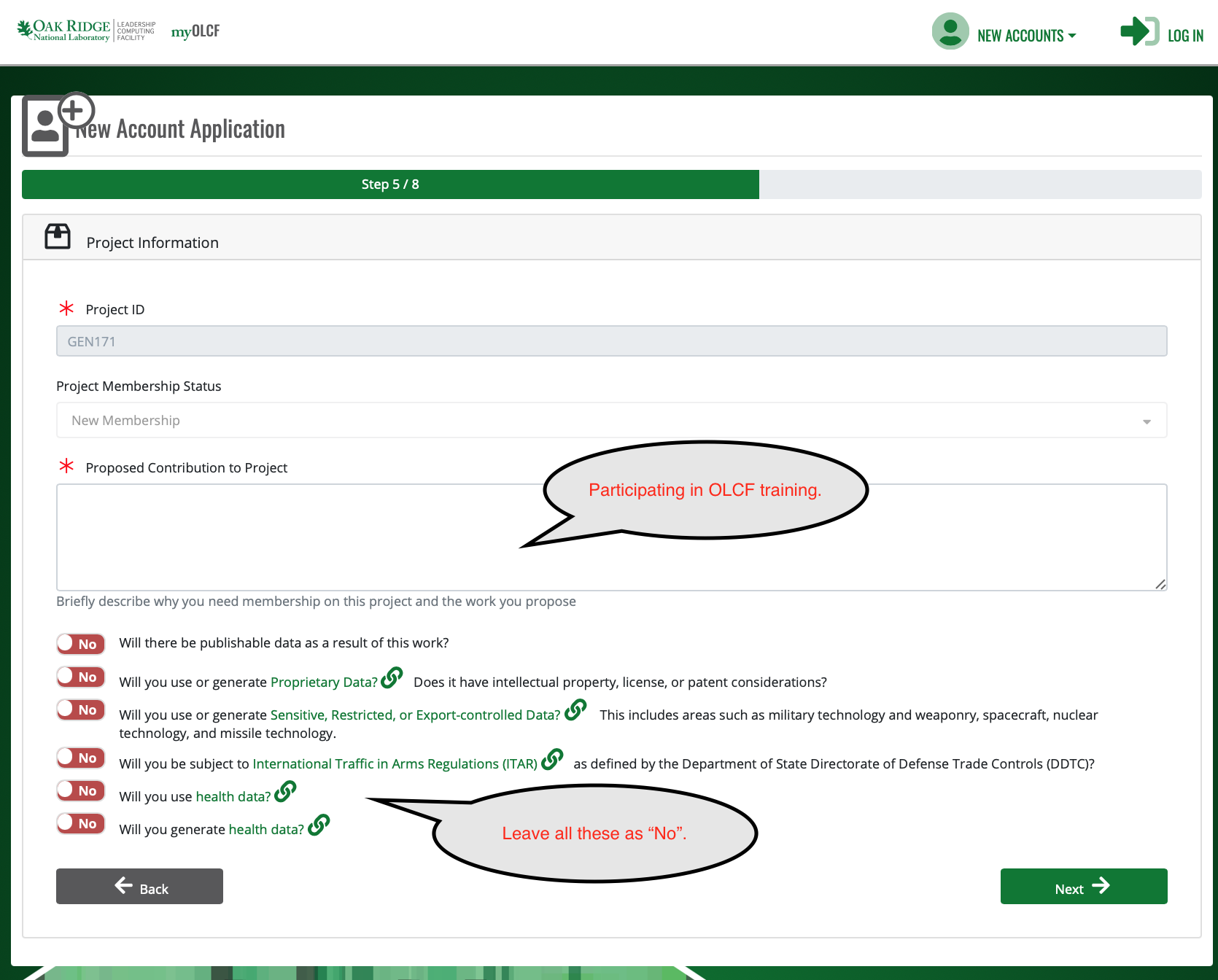
On the user account page, selected “yes” or “no” for the questions asking about any pre-existing account names. If this is your first account with us, leave those questions set to “no”. Also enter your preferred shell. If you do not know which shell to use, select “/bin/bash”. We can change this later if needed. Click “Next”.
On the “Policies & Agreements” page click the links to read the polices and then answer “Yes” to affirm you have read each. Certify your application by selecting “Yes” as well. Then Click “Submit.”
Note
After submitting your application, it will need to pass through the approval process. Depending on when you submit, approval might not occur until the next business day.
Step 2: Set Your XCAMS/UCAMS Password
Once approved, if you are a new user, your account will be created and an email will be sent asking you to set up a password. If you already had an XCAMS/UCAMS account, you will not be sent the email asking you to setup a new password (simply use your existing credentials). Once passwords are known, users can log in to Ascent using their XCAMS/UCAMS username and password (see the next section)
Logging In to Ascent
To log in to Ascent, please use your XCAMS/UCAMS username and password:
$ ssh USERNAME@login1.ascent.olcf.ornl.gov
Note
You do not need to use an RSA token to log in to Ascent. Please use your XCAMS/UCAMS username and password (which is different from the username and PIN + RSA token code used to log in to other OLCF systems such as Summit).
Note
It will take ~5 minutes for your directories to be created, so if your account was just created and you log in and you do not have a home directory, this is likely the reason.
Preparing For Frontier
This section of the Summit User Guide is intended to show current OLCF users how to start preparing their applications to run on the upcoming Frontier system. We will continue to add more topics to this section in the coming months. Please see the topics below to get started.
HIP
HIP (Heterogeneous-Compute Interface for Portability) is a C++ runtime API that allows developers to write portable code to run on AMD and NVIDIA GPUs. It is an interface that uses the underlying Radeon Open Compute (ROCm) or CUDA platform that is installed on a system. The API is similar to CUDA so porting existing codes from CUDA to HIP should be fairly straightforward in most cases. In addition, HIP provides porting tools which can be used to help port CUDA codes to the HIP layer, with no overhead compared to the original CUDA application. HIP is not intended to be a drop-in replacement for CUDA, so some manual coding and performance tuning work should be expected to complete the port.
Key features include:
HIP is a thin layer and has little or no performance impact over coding directly in CUDA.
HIP allows coding in a single-source C++ programming language including features such as templates, C++11 lambdas, classes, namespaces, and more.
The “hipify” tools automatically convert source from CUDA to HIP.
Developers can specialize for the platform (CUDA or HIP) to tune for performance or handle tricky cases.
Using HIP on Summit
As mentioned above, HIP can be used on systems running on either the ROCm or CUDA platform, so OLCF users can start preparing their applications for Frontier today on Summit. To use HIP on Summit, you must load the HIP module:
$ module load hip-cuda
CUDA 11.4.0 or later must be loaded in order to load the hip-cuda module. hipBLAS, hipFFT, hipSOLVER, hipSPARSE, and hipRAND have also been added to hip-cuda.
Learning to Program with HIP
The HIP API is very similar to CUDA, so if you are already familiar with using CUDA, the transition to using HIP should be fairly straightforward. Whether you are already familiar with CUDA or not, the best place to start learning about HIP is this Introduction to HIP webinar that was recently given by AMD:
More useful resources, provided by AMD, can be found here:
The OLCF is currently adding some simple HIP tutorials here as well:
OLCF Tutorials – Simple HIP Examples
Previous Frontier Training Events
The links below point to event pages from previous Frontier training events. Under the “Presentations” tab on each event page, you will find the presentations given during the event.
Frontier Application Readiness Kick-Off Workshop (October 2019)
Please check back to this section regularly as we will continue to add new content for our users.